10 L10: Improved Euler’s Method and Runge-Kutta Methods (3.2)
10.1 Recall Euler’s method
# Our differential equation
diff <- function(x,y)
{
return(x+y) #Try also x/y
}
# Line function
TheLine <- function(x1,y1,slp,d)
{
z = slope*(d-x1)+y1
return(z)
}
# Domains
x = seq(-20,20,0.5)
y = seq(-20,20,0.5)
# Points to draw our graph
f = c(-5,5)
h = c(-5,5)
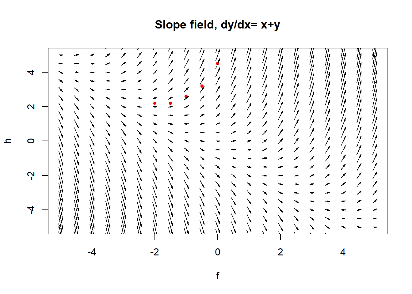
plot(f,h,main="Slope field, dy/dx= x+y")
lines(c(-2,-1.5,-1,-.5,0),c(2.2,2.2,2.6,3.2,4.5),type ="p",pch=19,cex=.7,col="red")
# Let's generate the slope field
for(j in x)
{
for(k in y)
{
slope = diff(j,k)
domain = seq(j-0.07,j+0.07,0.14)
z = TheLine(j,k,slope,domain)
arrows(domain[1],z[1],domain[2],z[2],length = 0.05, angle = 10,code=2)
}
}10.2 Recall Euler’s method (Zoom)
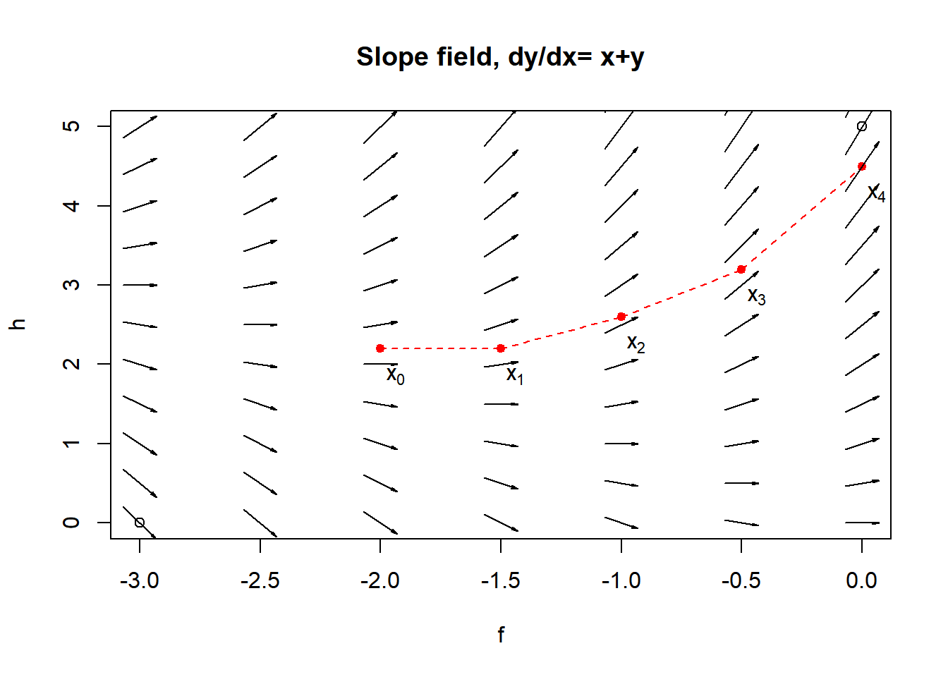
\[\frac{dy}{dx}=g(x,y),\qquad y(x_0)=y_0\] \[\boxed{y_1 = y_0+g(x_0,y_0)\cdot(x_1-x_0)}\]
How can we improve the method?
?
10.3 Improved linear approx.
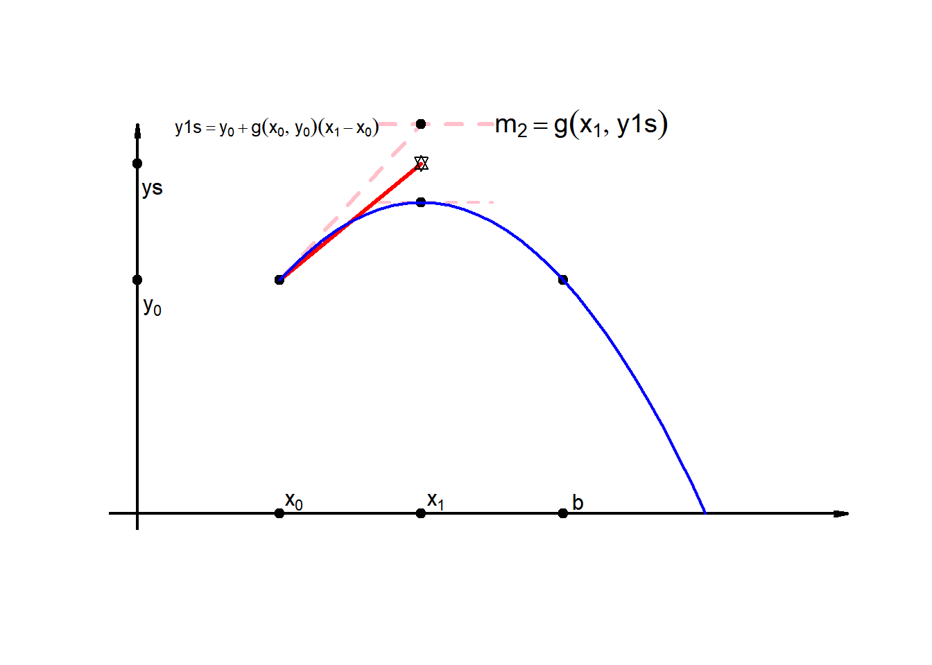
Conceptual Idea: use the slope at \((x_0,y_0)\) and the slope at \((x_1,y_1)\)
Concept: Average of the slopes to improve linear approximation.
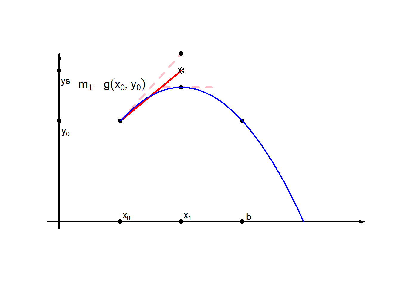
Calculate \(m_1\) by evaluating \(g(x_0,y_0\)), no problem!
Calculate \(m_2\) by evaluating \(g(x_1,y_1)\) \(\cdots\)
but I dont know \(y_1\), because that is what I want to find!
so what to do?
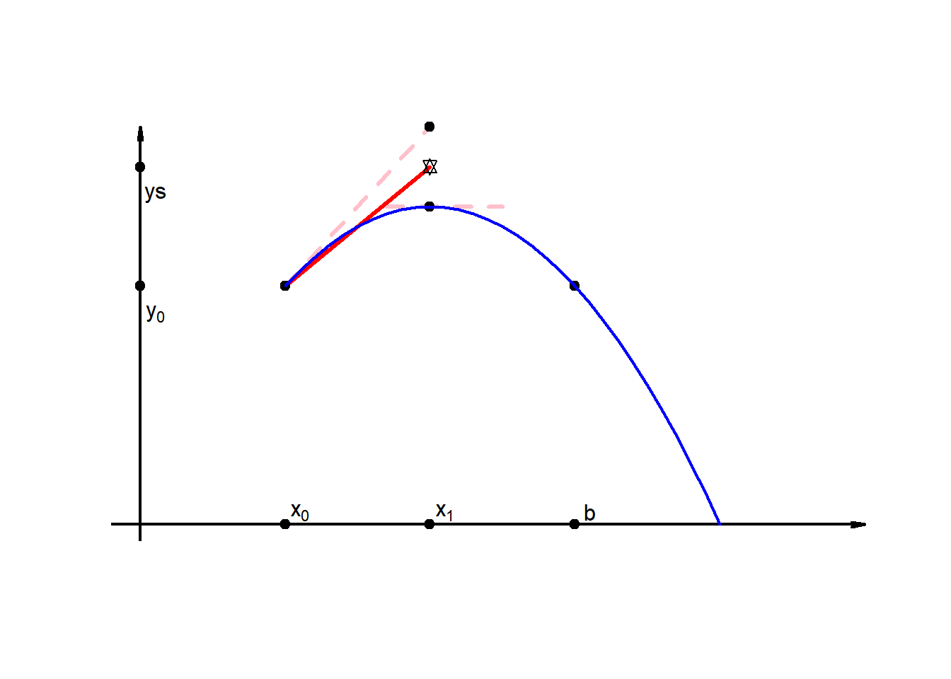
I can estimated \(y_1\)…
\[y_1 \approx y_0+g(x_0,y_0)(x_1-x_0)\] \[= y_{1s}\]
Now I use the average of \(m_1\) and \(m_2\) to get a better estimation of the function between \(x_0\) and \(x_1\):
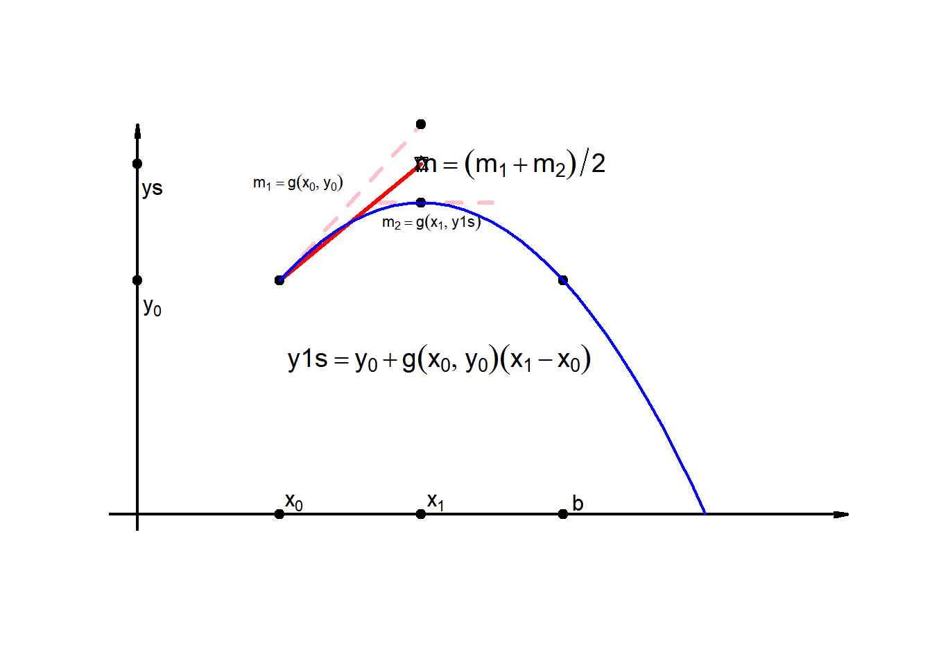
Improved linear approx.
10.4 1-step improved Euler
Idea: use slope at \((x_0,y_0)\) and \((x_1,y_1)\)
\[y_1^* = y_0+g(x_0,y_0)(x_1-x_0)\qquad\text{(1-step Euler)}\]
\[m=\frac{g(x_0,y_0)+g(x_1,y_1^*)}{2}\] \[\boxed{y_1=y_0+m(x_1-x_0)}\qquad\text{(Improved 1-step Euler)}\]
10.5 n-steps improved Euler1
\[\begin{align} y_1&=y_0+m_1(x_1-x_0)\\ y_2&=y_1+m_2(x_2-x_1)\\ \cdots \end{align}\]
\[\boxed{y_n=y_{n-1}+m_n(x_n-x_{n-1})}\] where \[m_n=\frac{g(x_{n-1},y_{n-1})+g(x_{n},y_n^*)}{2}\] and \(y_n^*\) is obtained with Euler method.
10.6 Runge-Kutta Methods
Second order method (weighted Improved Euler)
While Euler’s method is useful, it does quite poorly in cases where the solution is changing rapidly. A way to circumvent this is to adjust the value of \(\Delta x\) to be smaller, which comes at the expense of more computational time. A second way is to use a higher order solver than euler, and one such method is called the Runge-Kutta method.
\[\boxed{\boxed{y_1=y_0+aK_1+bK_2}}\] \[\boxed{K_1=g(x_0,y_0)\Delta x}\] \(K_1\), is defined as how much I rise when I only consider the rate at \(x_0\).
and
\[\boxed{K_2=g(x_0+\alpha\Delta x, y_0+\beta K_1)\Delta x}\] is defined as the rise due to the change of \(K_1\) and other parameters, \(\alpha\) and \(\beta\), which related how fast I am advancing on my immediate space.
The conditions for this parameters are:
\[\boxed{a+b=1,\qquad b\alpha=\frac{1}{2},\qquad b\beta =\frac{1}{2}}\] In most cases: \(\alpha=\beta=\frac{1}{2b}\)
10.7 Recovering Improved Euler from RK
\[\boxed{y_1=y_0+aK_1+bK_2}\]
But, if \[\alpha=1=\beta,\quad a=b=1/2\] then:
\[y_1=y_0+ag(x_0,y_0)\Delta x+bg(x_0+\alpha\Delta x, y_0+\beta K_1)\] \[y_1=y_0+\frac{1}{2}g(x_0,y_0)\Delta x+\frac{1}{2}g(x_0+\Delta x, y_0+K_1)\] \[y_1=y_0+\frac{1}{2}g(x_0,y_0)\Delta x+\frac{1}{2}g(x_0+\Delta x, y_0+\frac{1}{2}g(x_0,y_0)\Delta x)\] \[ \boxed{y_1 = y_0+\frac{g(x_0,y_0)+g(x_1,y_1)}{2}\Delta x} \]
10.8 A popular Fourth-order RK
To illustrate how the Runge-Kutta 4th order (RK4) method works, let’s consider a simple differential equation that we can solve numerically. The RK4 method is a popular method for solving ordinary differential equations (ODEs) numerically because it offers a good balance between accuracy and computational efficiency. It approximates the solution by taking the weighted average of four increments, where each increment provides an estimate of the slope.
Let’s take a differential equation of the form:
\[\frac{dy}{dx} = f(x, y)\]
And we want to solve this equation over an interval from \(x = x_0\) to \(x = x_n\), given an initial condition \(y(x_0) = y_0\).
The RK4 method computes the next value \(y_{n+1}\) based on the current value \(y_n\) using the formula:
\[y_{n+1} = y_n + \frac{1}{6}(k_1 + 2k_2 + 2k_3 + k_4)\]
where:
- \(k_1 = h \cdot f(x_n, y_n)\)
- \(k_2 = h \cdot f(x_n + \frac{1}{2}h, y_n + \frac{1}{2}k_1)\)
- \(k_3 = h \cdot f(x_n + \frac{1}{2}h, y_n + \frac{1}{2}k_2)\)
- \(k_4 = h \cdot f(x_n + h, y_n + k_3)\)
And \(h\) is the step size.
10.8.1 Example
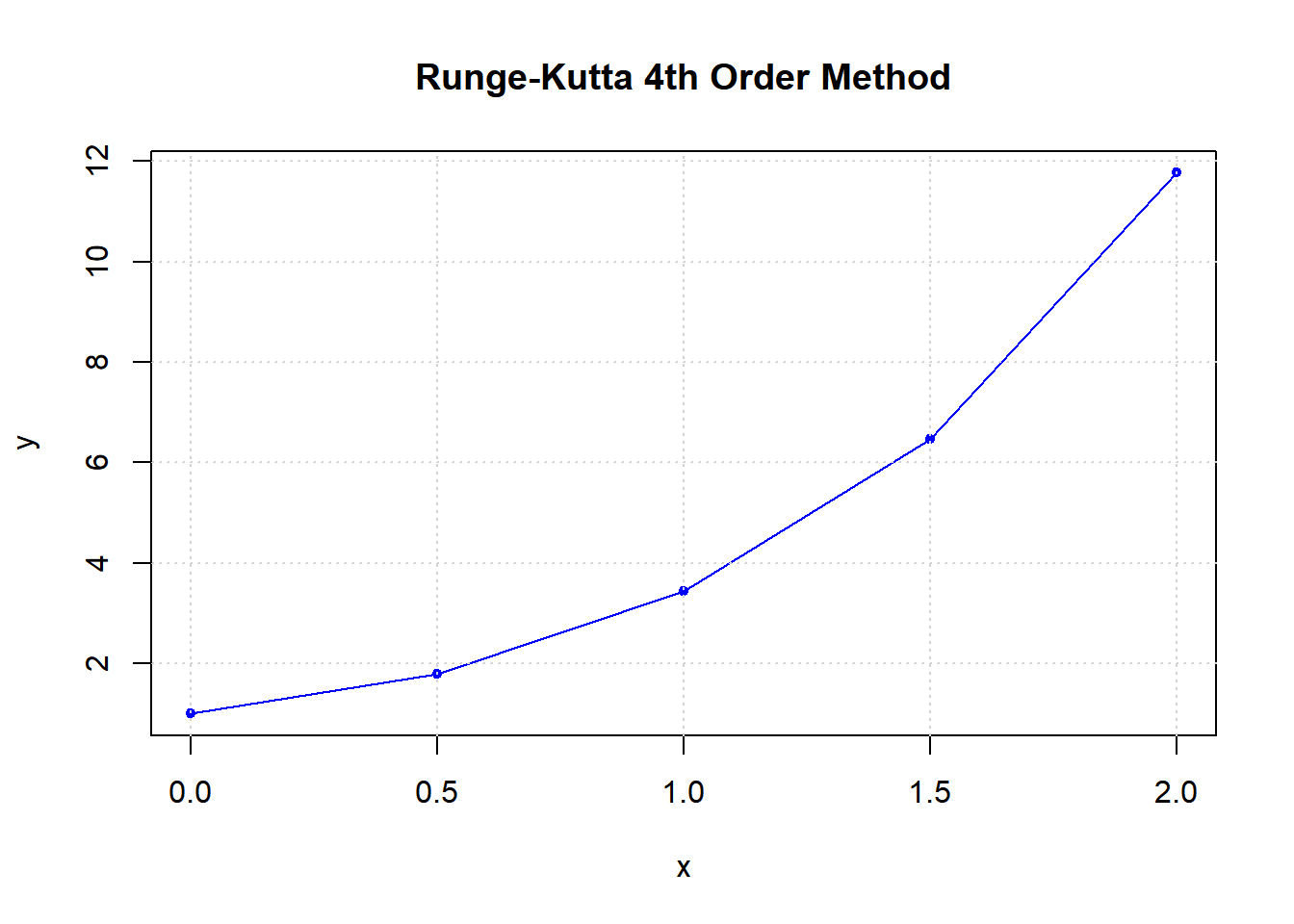
To demonstrate this visually, let’s solve a simple ODE, such as \[\frac{dy}{dx} = x + y\] with the initial condition \(y(0) = 1\) over the interval \(0 \leq x \leq 2\), using a step size \(h = 0.5\).
I’ll plot the approximation at each step to show how RK4 method progresses. Let’s start by implementing this.
# Define the differential equation
f <- function(x, y) {
  x + y
}

# Implement RK4 method
rk4 <- function(x0, y0, x_end, h) {
  n <- as.integer((x_end - x0) / h)
  x <- x0
  y <- y0
  xs <- c(x)
  ys <- c(y)

  for (i in 1:n) {
    k1 <- h * f(x, y)
    k2 <- h * f(x + 0.5 * h, y + 0.5 * k1)
    k3 <- h * f(x + 0.5 * h, y + 0.5 * k2)
    k4 <- h * f(x + h, y + k3)

    y <- y + (k1 + 2 * k2 + 2 * k3 + k4) / 6
    x <- x + h

    xs <- c(xs, x)
    ys <- c(ys, y)
  }

  list(x = xs, y = ys)
}

# Initial conditions
x0 <- 0
y0 <- 1
x_end <- 2
h <- 0.5

# Solve ODE
solution <- rk4(x0, y0, x_end, h)

# Plotting
plot(solution$x, solution$y, type = 'o', col = 'blue', xlab = 'x', ylab = 'y',
     main = 'Runge-Kutta 4th Order Method', pch = 20)
grid()
To run this script, you’ll need an R environment set up, such as RStudio or a Jupyter notebook with an R kernel. This script follows the steps outlined:
- It first defines the differential equation you’re solving.
- Then, it implements the RK4 method, iterating over the interval [x0, x_end] with steps of size h, and calculates y values at each step.
- Finally, it plots the (x, y) points using the base plotting system in R, highlighting the RK4 approximation of the solution to the differential equation.
The plot above demonstrates how the Runge-Kutta 4th order (RK4) method approximates the solution to the differential equation \(\frac{dy}{dx} = x + y\) with the initial condition \(y(0) = 1\), over the interval \(0 \leq x \leq 2\), using a step size \(h = 0.5\). Each point on the plot represents the value of \(y\) at a given \(x\), calculated using the RK4 method. This method takes four slope estimates (\(k_1\), \(k_2\), \(k_3\), \(k_4\)) at each step and uses their weighted average to achieve a high level of accuracy with relatively few steps.
10.9 Example using demodelr
10.10 Using Runge-Kutta-4 function from R
rm(rk4) # First I need to remove my rk4 function
library(demodelr) # This library load a rk4, and more

infection_eq <- c(dpdt ~ .023 * p * (1 - p))
prop_init <- c(p = 250/13600)
deltaT <- 1
n_steps <- 600
out_solution <- rk4(system_eq = infection_eq,
                      initial_condition = prop_init,
                      parameters = c(beta=0.2, alpha=0.2),
                      deltaT = deltaT,
                      n_steps = n_steps
)str(out_solution)tibble [600 × 2] (S3: tbl_df/tbl/data.frame)
$ t: num [1:600] 0 1 2 3 4 5 6 7 8 9 ...
$ p: num [1:600] 0.0184 0.0188 0.0192 0.0197 0.0201 ...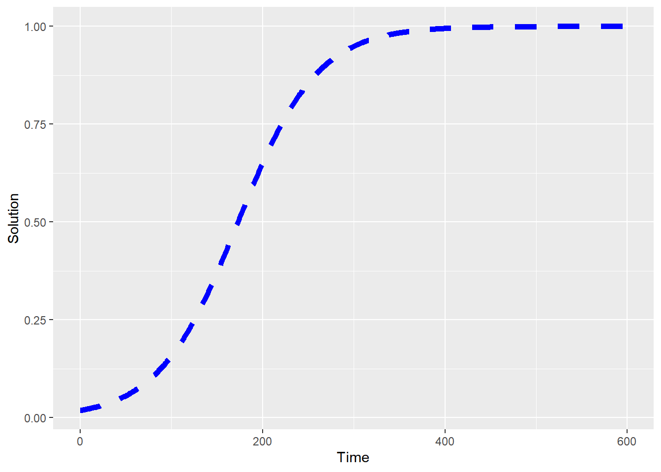
library(ggplot2)
ggplot(data = out_solution) +
  geom_line(aes(x = t, y = p), color = "blue",linetype='dashed', lwd=2) +
  labs(
    x = "Time",
    y = "Solution"
  )
10.11 References
please put attention, for n-steps \(m_1\) is not the same of 1-step Euler. \(m_1\) correspond to the mean of the slope at \(x_0\) and \(x_1\).↩︎