9 L9: Euler’s Method (3.1)
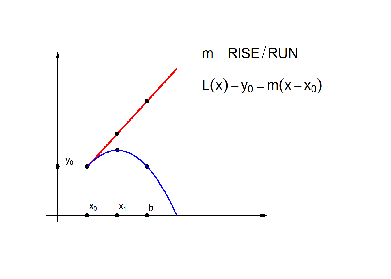
9.1 Linear approx.(1-Step-Euler)
Suppose we are given:
\[\frac{dy}{dx}=g(x,y),\qquad y(x_0)=y_0\]
\[x_0\leq x \leq b\] and we want to know \(y(x_1)\) where \(x_1>x_0\)
\[L(x)=y_0+m\cdot(x-x_0)\] \[L(x)=y_0+g(x_0,y_0)\cdot(x-x_0)\]
\[\therefore \boxed{y \approx y_0+g(x_0,y_0)\cdot(x-x_0)}\]
9.2 Linear approx.(2-Step-Euler)
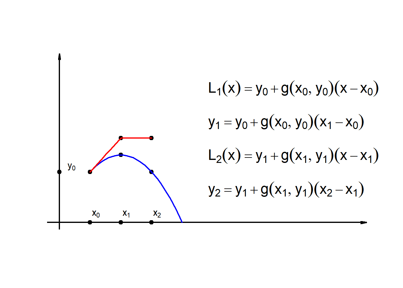
\[L_1(x) = y_0+g(x_0,y_0)(x-x_0)\] \[y_1(x) = y_0+g(x_0,y_0)(x_1-x_0)\] \[L_2(x) = y_1+g(x_1,y_1)(x-x_1)\] \[y_2(x) = y_1+g(x_1,y_1)(x_2-x_1)\]
9.3 Euler’s method (n-steps)
Approximate: \[y(x^*),\qquad\text{where }\quad x_0\leq x^* \leq b\]
given: \[\boxed{\frac{dy}{dx}=g(x,y)},\qquad y(x_0)=y_0\]
\[\begin{align} L_1(x)&=y_0+g(x_0,y_0)(x-x_0)\\ y_1=L_1(x_1)&=y_0+g(x_0,y_0)(x_1-x_0)\\ L_2(x)&=y_1+g(x_1,y_1)(x-x_1)\\ y_2=L_2(x_2)&=y_1+g(x_1,y_1)(x_2-x_1)\\ L_3(x)&=y_2+g(x_2,y_2)(x-x_2)\\ y_3=L_3(x_3)&=y_2+g(x_2,y_2)(x_3-x_2)\\ \cdots\\ L_n(x)&=y_{n-1}+g(x_{n-1},y_{n-1})(x-x_{n-1})\\ y_n=y(x^*)&=L_n(x_n)\\ &=y_{n-1}+g(x_{n-1},y_{n-1})(x_n-x_{n-1}) \end{align}\]
Note:
As \(n\rightarrow \infty\), Error \(\rightarrow 0\)
In practice we use high-level language, like R, python, etc.
Also we can use calculator, in an iterative way.
Let’s revise a couple of examples using R.
y <- function(x){cos(x)}
dydx <- function(x){-sin(x)}
x0 <- 0
xgoal <- pi/2
n <- 10
y0 <- y(x0) #initial condition we do know
L1 <- function(x){y0 + dydx(x0)*(x-x0)}
x1 <- x0+1/n*(xgoal-x0)
y1 <- L1(x1)
L2 <- function(x){y1 + dydx(x1)*(x-x1)}
x2 <- x0+2/n*(xgoal-x0)
y2 <- L2(x2)
L3 <- function(x){y2 + dydx(x2)*(x-x2)}
x3 <- x0+3/n*(xgoal-x0)
y3 <- L3(x3)
L4 <- function(x){y3 + dydx(x3)*(x-x3)}
x4 <- x0+4/n*(xgoal-x0)
y4 <- L4(x4)
plot(y, col="blue")
lines(c(x0,x1,x2,x3,x4),c(y0,y1,y2,y3,y4), col="red")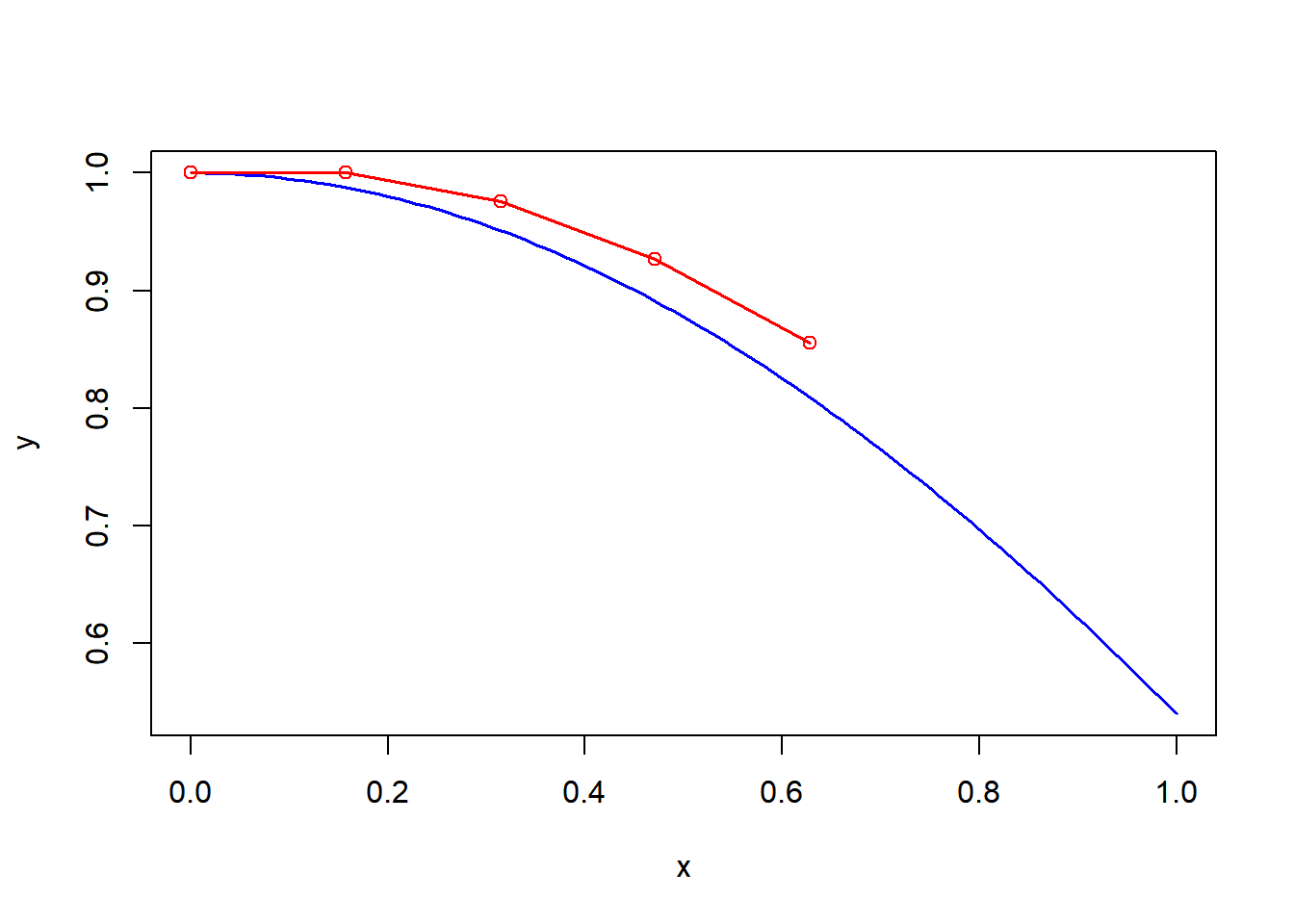
9.4 Using Euler function from R
- In a high-level language, there are so many functions already defined, no need to reinvent the wheel!
- We just need to find a good library:
library(demodelr)Registered S3 method overwritten by 'GGally':
method from
+.gg ggplot2infection_eq <- c(dpdt ~ .023 * p * (1 - p))
prop_init <- c(p = 250/13600)
deltaT <- 1
n_steps <- 600
out_solution <- euler(system_eq = infection_eq,
initial_condition = prop_init,
deltaT = deltaT,
n_steps = n_steps
)The output is a dataframe.
#summary(out_solution)
str(out_solution)
tibble [600 × 2] (S3: tbl_df/tbl/data.frame)
$ t: num [1:600] 0 1 2 3 4 5 6 7 8 9 ...
$ p: num [1:600] 0.0184 0.0188 0.0192 0.0197 0.0201 ...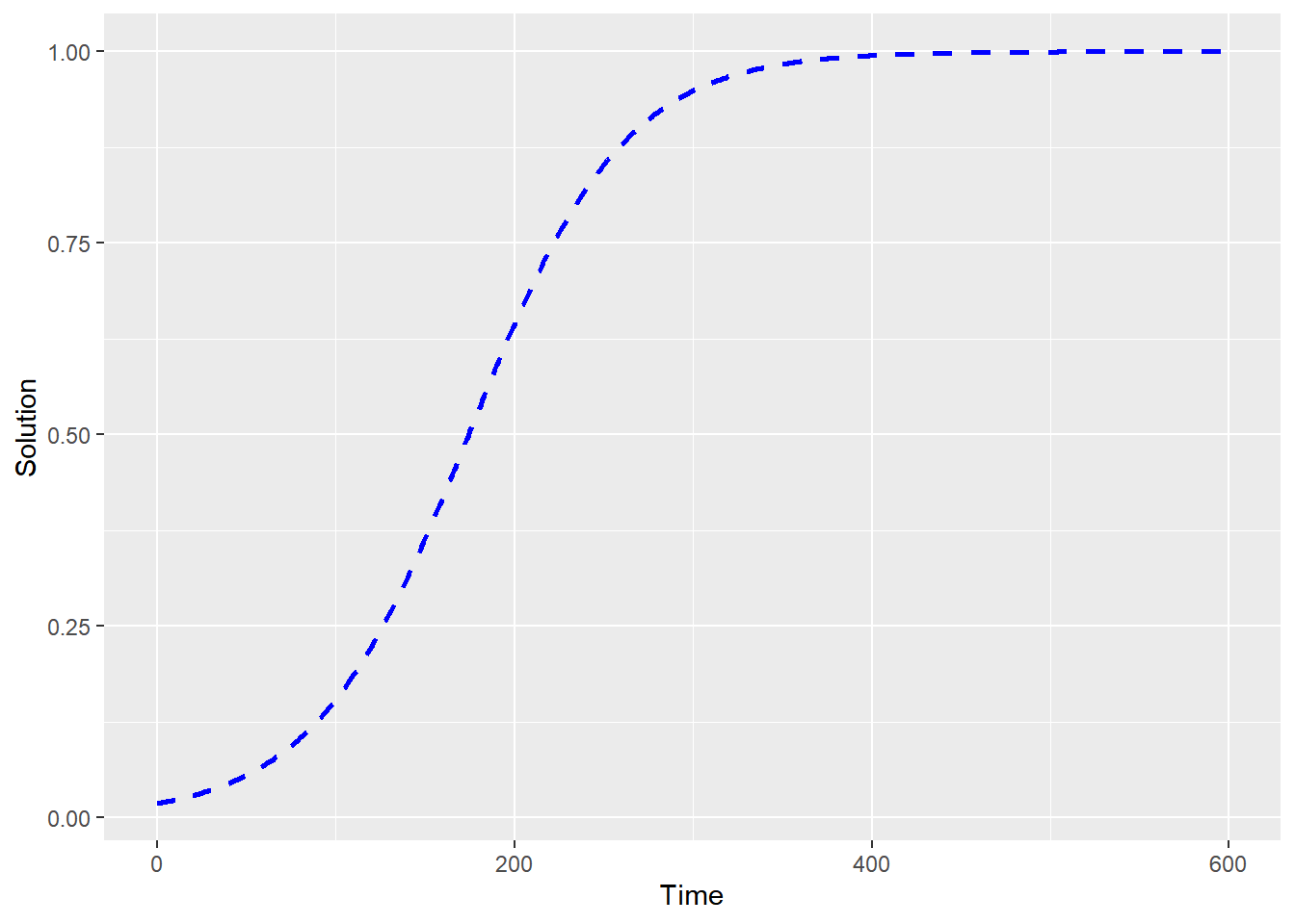
library(ggplot2)
ggplot(data = out_solution) +
  geom_line(aes(x = t, y = p), color = "blue",linetype='dashed', lwd=1.5) +
  labs(
    x = "Time",
    y = "Solution"
  )