3 L3: Direction Fields
3.1 ODE Direction Fields
Graphing solutions to 1\(^{st}\) order differential equations (ODE)
Direction Fields:
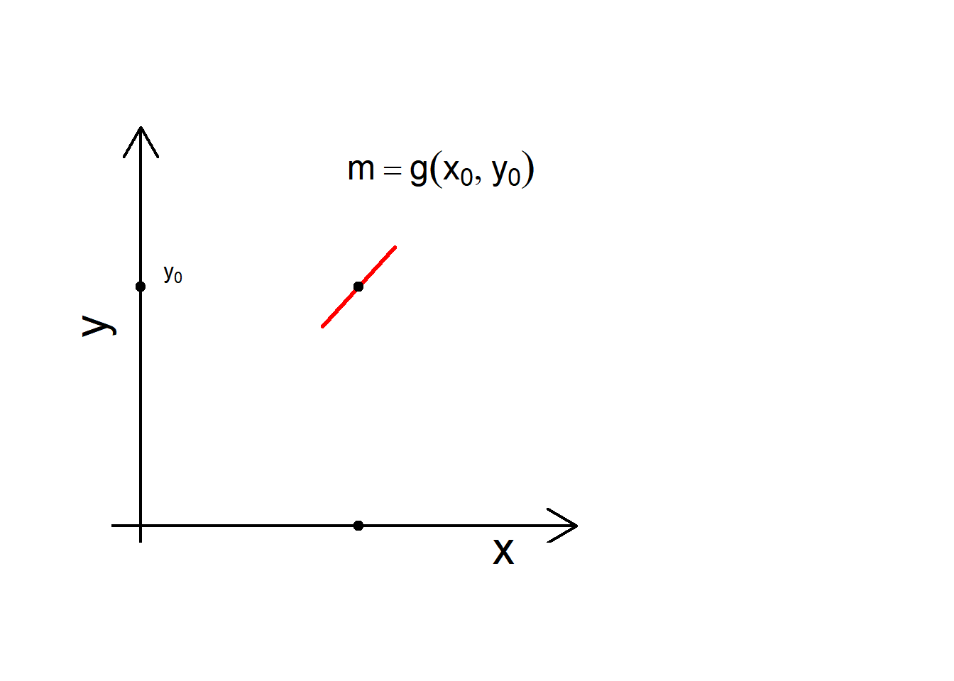
Suppose \[\frac{dy}{dx}=g(x,y)\] and \[y(x_0)=y_0\]
What to do?
a segment with slope \(g(x_0,y_0)\) for each coordinate \((x_0,y_0)\):
Example. Let’s work it out an example by hand and then with r-code
\[\frac{dy}{dx}=ky;\quad k>0\]
Solution
Let’s plot by hand \(\frac{dy}{dx}=ky\) in the \(x-y\) plane, assume a value for \(k\) :
We do know how to find a solution for our differential equation:
\[\begin{align} \frac{dy}{dx}&=ky\\ \int\frac{dy}{y}&=\int kdx\\ \ln |y| &= kx+C\\ |y|&=D_0e^{kx},\quad D_0>0\\ y&=y_0e^{kx} \end{align}\]
If the initial condition is: \[y(0)=0\], how do look a solution in our direction field?
we could use online solvers: https://www.wolframalpha.com/input?i=direction+field+dy%2Fdx+%3D+3*y
Like playing pinball…
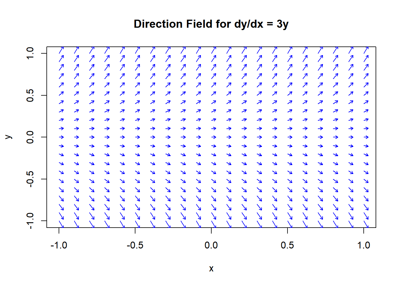
dydx <- function(x, y) {
return(3 * y)
}
# Create a sequence of x values
x_values <- seq(from = -1, to = 1, by = 0.1)
# Initialize an empty plot
plot(NA, xlim = c(-1, 1), ylim = c(-1, 1), xlab = "x", ylab = "y", main = "Direction Field for dy/dx = 3y")
# Loop over x and y values to draw the direction field
for (x in x_values) {
for (y in x_values) {
# Solve the differential equation at this point
slope <- dydx(x, y)
# Calculate a small step along the direction of the field
dx <- 0.03
dy <- slope * dx
# Draw an arrow to represent the direction field
arrows(x0 = x, y0 = y, x1 = x + dx, y1 = y + dy, col = "blue", length = 0.05)
}
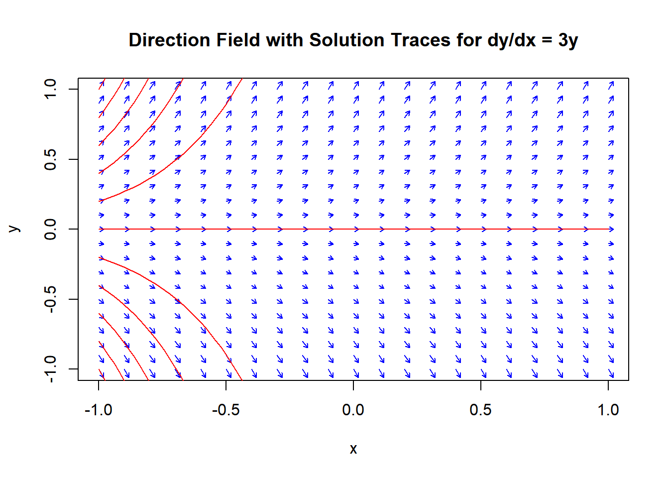
}\[\frac{dy}{dt}=3y,\qquad y(0)=0.5\]
# Load the deSolve package
library(deSolve)

# Define the differential equation
ode_function <- function(t, y, parameters) {
  dy <- 3 * y
  list(dy)
}

# Initial condition
y0 <- 0.5

# Time (x) points at which solution is sought
time <- seq(from = 0, to = 5, by = 0.1)

# Solve the differential equation
sol <- ode(y = y0, times = time, func = ode_function, parms = NULL)

# Plot the solution
plot(sol, main = "Solution of dy/dt = 3y", xlab = "t", ylab = "y", type = "l")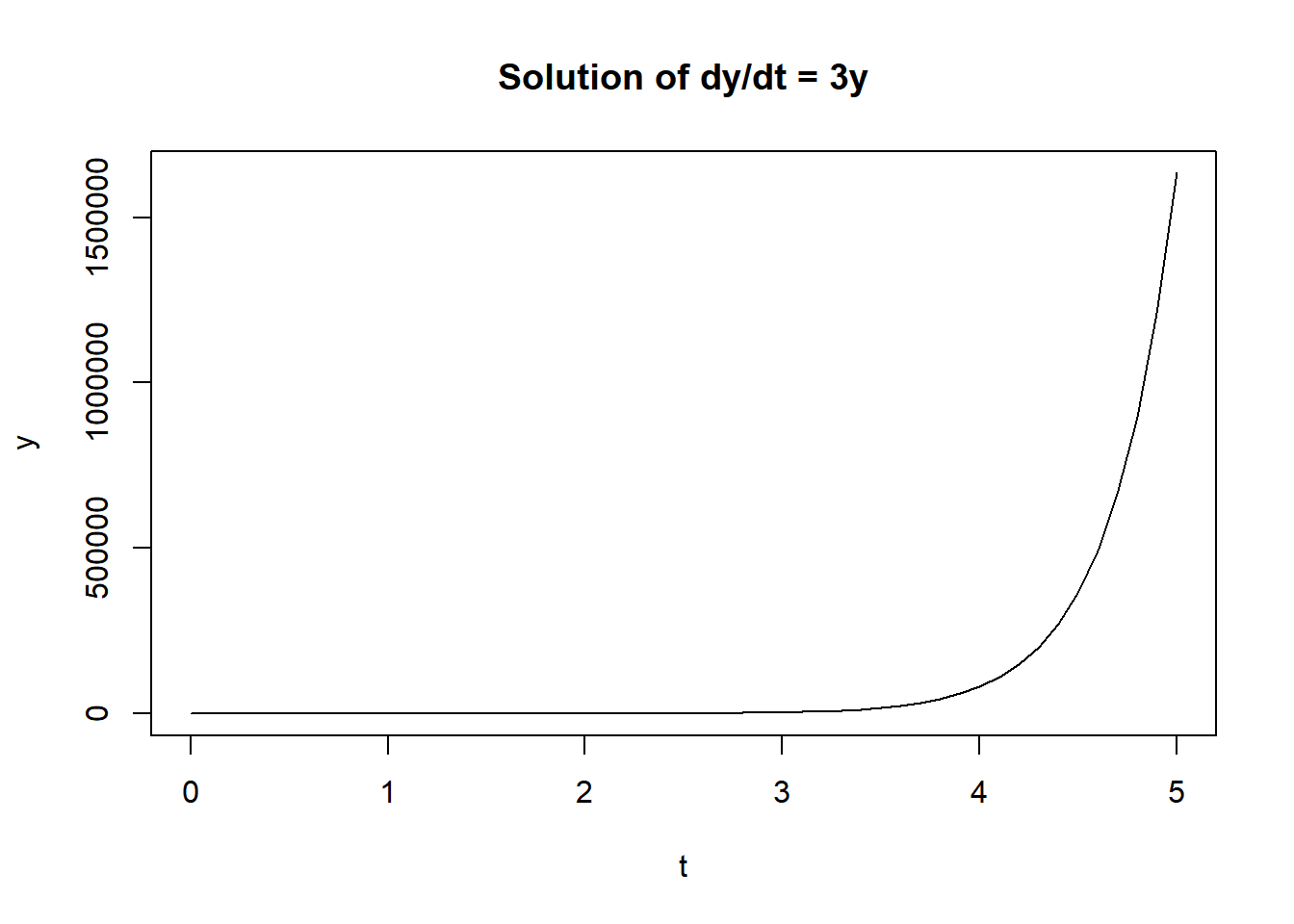
Let’s put all together, including a few particular solutions:
3.2 Direction Field definitions
Definition: Direction Field jargon
- A
solution curveis tangent to the direction field lines at each point.
- An
isoclineis the set of all points in the \(xy\)-plane that are associated with a constant slope \(C\).
Example
from wiki1 \[\frac{dy}{dx}=xy\] Blue: isocline; Black: Slope field; Red: Some solutions

3) In the graph of \(\frac{dy}{dx}\) versus \(y\), points \(y\) for which \(\frac{dy}{dx}=0\) are called rest points, equilibrium points, or critical points.
3.3 Let’s remember problem last class
Example: Falling body with viscous friction

- Assumptions: \(h<<R_E\) and viscous friction for air resistance.
Solution
\[\begin{align} \sum F &= m\frac{dv}{dt}\\ -kv+mg &=m\frac{dv}{dt}\\ \frac{dv}{dt}&=\frac{mg-kv}{m}\\ \int \frac{m}{mg-kv}\,dv&=\int dt\\ \text{change of variables}&:(mg-kv=u\rightarrow-kdv=du)\\ \frac{m}{-k}\int \frac{1}{u}\,du &= t+C\\ \ln |u| &= -\frac{k}{m}(t+C)\\ \ln |mg-kv| &= -\frac{k}{m}(t+C)\\ mg-kv &=e^{-kt/m}\cdot e^C\\ kv &=mg-e^{-kt/m}\cdot e^C \end{align}\]
\[\boxed{v=\frac{1}{k}\left(mg-e^{-kt/m}\cdot e^C\right)}\] If initial conditions are: \(\boxed{v(0)=0}\) then:
\[\begin{align} 0&=\frac{1}{k}\left(mg-e^{0}\cdot e^C\right)\\ 0&=\frac{1}{k}\left(mg-1\cdot e^C\right)\\ \Rightarrow\\ C&= \ln (mg)\\ \Rightarrow\\ v&=\frac{1}{k}\left(mg-e^{-kt/m}\cdot (mg)\right) \end{align}\]
Finally:
\[\boxed{v=\frac{mg}{k}\left(1-e^{-kt/m}\right)}\]
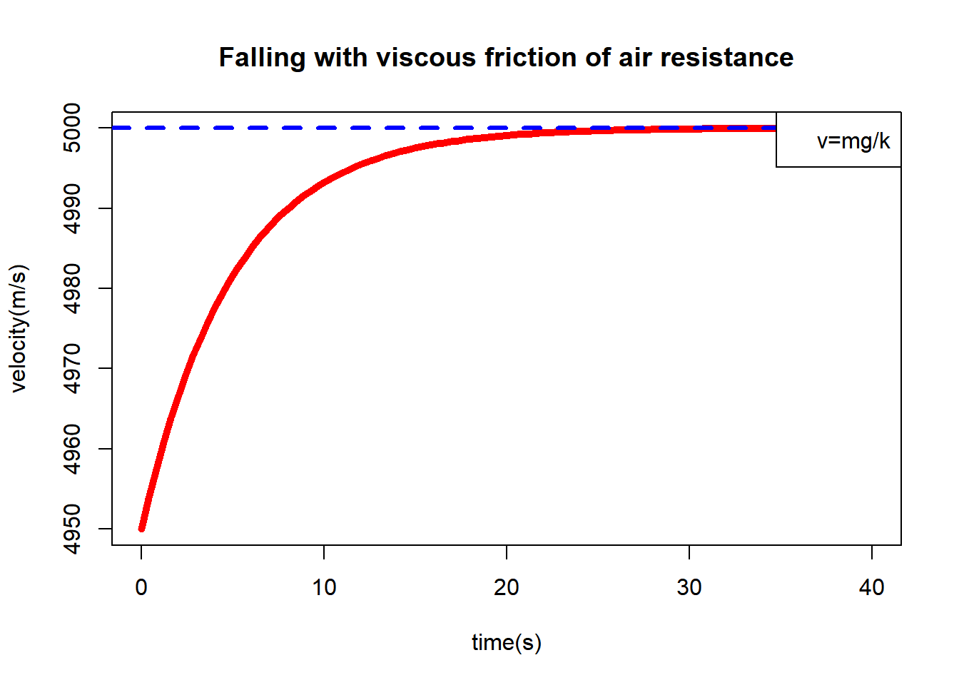
3.3.1 Plot for terminal velocity:
at terminal velocity: \[t\rightarrow \infty\qquad(\text{or } t>>m/k)\] \[\Rightarrow\] \[\boxed{v=\frac{mg}{k}\left(1-e^{-kt/m}\right) \rightarrow \frac{mg}{k}(1-0)}\]
\[\boxed{v_{terminal}=\frac{mg}{k}}\]
```{r,echo=TRUE}
m <- 100
g <- 10
k <- .2
t <- seq(0, 40, length.out = 100)
v <- m*g/k*(1-exp(-k*t)/m)
#vterm <- rep(m*g/k, each=100)
plot(t,v, type="l", col="red", lwd=5, xlab="time(s)", ylab="velocity(m/s)", main="Falling with viscous friction of air resistance")
#lines(t, vterm, type="d", col="blue", lwd=2)
abline(h=m*g/k, col = "blue",lwd=3, lty=2)
legend("topright", legend= "v=mg/k")
```
3.4 Example maxima-cas
Directional Field, critical points:
\[\boxed{\frac{dv}{dt}=\frac{mg-kv}{m}}\]
Solution
m :100;
g: 10;
k: 20;(%i1) dvdt: (100*10-20*y)/100$
(%i2) plotdf(dvdt,[trajectory_at,0,0],[ycenter,50],[yradius,50],[xradius,50]);(%o2) "C:/Users/evalderrama/AppData/Local/Temp/maxout16368.xmaxima"\[\boxed{v_{terminal}=\frac{mg}{k}}\]
3.5 Stability of Critical Points
Definitions:
Let
\[\boxed{\frac{dy}{dx}=g(x,y)} \tag{3.1}\]
and let \(y_0\) be a critical point for the differential equation.
The critical point is said to be:
1) Stable:
If for every number \(\varepsilon >0\) there is a number \(\delta>0\) such that whenever \[|y_0-y(0)|<\delta\] where \(y\) is a solution to (Equation 3.1)
we have: \[|y_0-y(t)|<\varepsilon\] for all \(t\geq T\)
2) asymptotically Stable:
If it is stable and there exists a number \(A>0\) such that whenever \[|y_0-y|<A\] we have
\[\lim_{t\rightarrow \infty }|y_0-y(t)|=0\]
3) unstable:
If it is not stable.
3.6 Example maxima-cas
Example
Show that the critical points for \[\frac{dy}{dt}=y^3(y^2-4)\] are \[\boxed{y_0=2},\quad \boxed{y_0=-2},\quad \boxed{y_0=0}\]
Solution
(%i3) dydt: y^3*(y^2-4)$
(%i4) plotdf(dydt,[trajectory_at,0,-2],[ycenter,0],[yradius,3],[xcenter,2],[xradius,4]);
(%o4) "C:/Users/evalderrama/AppData/Local/Temp/maxout16368.xmaxima"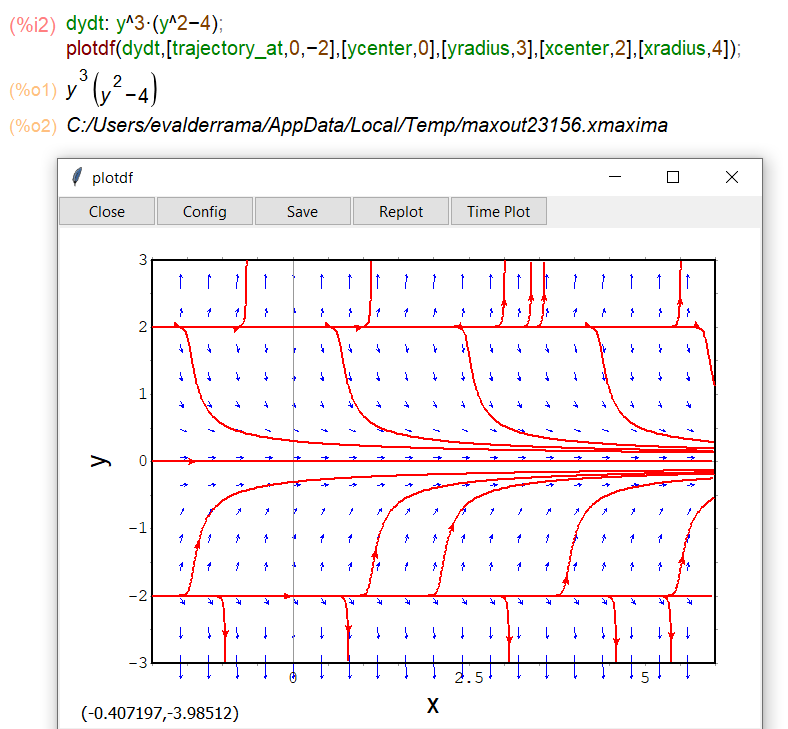
Intuitively, a critical point \(y=y_0\) of a first order equation is said to be stable provided that, if the initial value is sufficiently close to \(y_0\), then the solution \(y(t)\) remains close to \(y_0\), for all \(t>0\). Otherwise, the critical point \(y_0\) is considered to be unstable. In other words unstable means that no matter how close to \(y_0\) your initial value is, the solution \(y(t)\) becomes not close to \(y_0\), for some \(t>0\).
3.7 Wolfram Alpha Examples
Tip
\[\frac{dy}{dx}=x+y\] https://www.wolframalpha.com/input?i=direction+field+dy%2Fdx+%3D+x%2By
- direction field dy/dx = x*y
- direction field dy/dx = sin(x*y)
Check this link for codes in different programming languages: https://en.wikipedia.org/wiki/Slope_field
3.8 Geogebra
Also eeeasy using another online interactive tool!
Let’s play!
3.9 Have questions ?
Schedule Office Hours with your Instructor Here!
3.10 References
- Slope Field (aka Direction Field) https://en.wikipedia.org/wiki/Slope_field
plotdfusing maxima-cas. https://maths.cnam.fr/Membres/wilk/MathMax/help/Maxima/maxima_68.html- Quarto revealjs. https://quarto.org/docs/presentations/revealjs/themes.html
https://en.wikipedia.org/wiki/Isocline↩︎