n <- 199
m <-  20
nE <- n-m+1
paste("The total number of events is n(E)=", nE)
[1] "The total number of events is n(E)= 180"Lets’ start with some basics definitions and examples:
Probability is a measure of the likelihood or chance that a specific event will occur. It quantifies the uncertainty associated with different outcomes in situations where multiple possibilities are present.
Maybe a simple example will illustrate this better:
If you need to guess,
What is the likelihood of rolling the number three on a fair six-sided dice in a single roll?
The number three appears on just one out of the six faces: \[\frac{1}{6}\] Now, when you roll the dice, there’s an equal chance of it landing on any of those numbers. So, since there is only one face with the number three, you have a 1 in 6 chance of rolling a three. Then the probability of rolling the number 3 in a single dice roll is \(\frac{1}{6}\), which is approximately 17%.
Defining two key concepts will be helpful: the Sample Space and the concept of an Event.
A sample space is the set of all possible outcomes of a random process or experiment. An event is a subset of a sample space.
The sample space correspond to all possibles outcomes, i.e.
\[S=\{(1,1),(1,2),(1,3),(1,4),\] \[\qquad (2,1),(2,2),(2,3),(2,4),\] \[\qquad (3,1),(3,2),(3,3),(3,4),\] \[\qquad (4,1),(4,2),(4,3),(4,4)\}\]
If \(E\) represent the event of the sum be equal to 4, there are 3 possibilities:
\[E=\{(1,3), (2,2), (3,1)\}\]
Now there are 3 events that provide the desire outcome, and from the previous problem I know that there are 16 possible total outcomes, then an educated guess said that the probability is the ratio between these two quantities: \[\frac{3}{16}\approx 19\%\]
Now we could provide a conjecture of what would the the formula to calculate the probability of a event
In the context of a finite sample space S where all outcomes are equiprobable, and E represents an event within this sample space, the probability of event E can be calculated using the following formula:
\[\boxed{P(E) = \frac{n(E)}{n(S)}}\]
Here, n(A) denotes the cardinality of set A, which represents the number of elements in set A.
Note: The resulting probability value, denoted as P(E), always falls within the range of 0 to 1, with P(E) = 0 indicating impossibility and P(E) = 1 indicating certainty.
What is the probability of rolling an even number on a standard 6-sided die.
If a Dodecahedron is rolled once, what is the probability that the outcome is greater than 9?
\[P(even)=\frac{n(E)}{n(S)}=\frac{n(\{2,4,6\})}{n(\{1,2,3,4,5,6\})}=\frac{3}{6}=50\%\]
\[E=\{10,11,12\}\] \[\Rightarrow\] \[P(x>9)=\frac{n(E)}{n(S)}=\frac{3}{12}=25\%\]
If \(m,n\in \mathbb{Z}\) and \(m\leq n\), then there are \(n-m+1\) integers from \(m\) to \(n\) inclusive.
\[100,\quad 105,\quad 110,\quad \cdots,\quad995\] \[=20\times 5,\quad 21\times 5,\quad 22\times 5,\quad \cdots,\quad 199\times 5\] \[\Rightarrow\]
n <- 199
m <- 20
nE <- n-m+1
paste("The total number of events is n(E)=", nE)[1] "The total number of events is n(E)= 180"\[P=\frac{n(E)}{n(S)}\]1
nS <-  999-100+1
P <- nE/nS
paste("The probability that a three digit integer is divisible by 5 is:", 100*P,"%")
[1] "The probability that a three digit integer is divisible by 5 is: 20 %"In combinatorics, determining the total number of outcomes for a sequence of events involves a fundamental rule known as the multiplication principle. This principle applies universally to scenarios with multiple steps or stages, allowing the calculation of the total possible outcomes by considering each stage individually.
General Rule:
The multiplication principle dictates that the total number of possible outcomes for a sequence of events is obtained by multiplying the number of choices at each stage.
Suppose you have:
Regardless of whether the events are independent or dependent, the total outcomes for the sequence of events are calculated using the formula:
\[ \text{Total outcomes} = n_1 \cdot n_2 \cdot n_3 \cdot \ldots \]
This rule remains consistent, accounting for both independent events (where the outcome of one event does not influence the others) and dependent events (where the outcomes are interconnected and influenced by previous events). For dependent events, the number of choices for each subsequent event may vary based on the outcomes of the prior events, yet the multiplication principle still applies uniformly to derive the total possible outcomes.
A PIN number consists of four digits(0-9) in sequence
Each Event is not affected by the next event, so each of them have 10 choices (0-9), then:
n1 <- 10
n2 <- 10
n3 <- 10
n4 <- 10
nS <- n1*n2*n3*n4
paste("The total number of possible combinations for PINS is:",nS)
[1] "The total number of possible combinations for PINS is: 10000"The initial event provides 10 choices, but for subsequent events, one option is eliminated due to the constraint of not being able to select what was chosen in the preceding step. This pattern continues in the following steps:
n1 <- 10
n2 <- 9
n3 <- 8
n4 <- 7
nE <- n1*n2*n3*n4
paste("The total number of possible combinations for PINS with NO repetition is:",nE)
[1] "The total number of possible combinations for PINS with NO repetition is: 5040"This was a guided problem, previous parts was designed to calculate the values I need for this part:
paste("The probability that a randomly chosen PIN contains no repetitions is:",round(100*nE/nS,1),"%")[1] "The probability that a randomly chosen PIN contains no repetitions is: 50.4 %"The addition rule in probability deals with the likelihood of either one event or another event occurring. It’s particularly useful when events are mutually exclusive, meaning they cannot happen simultaneously. The rule states that the probability of either Event A or Event B occurring is the sum of their individual probabilities:
\[\boxed{P(A \text{ or } B) = P(A\cup B)=P(A) + P(B)}\]
What is the probability that numbers from 1-999 do not have any repeated digits?
In order to apply the addition rule in this context, we must identify events that are mutually exclusive, essentially sets that are non-overlapping. For instance, in this particular problem, we can distinguish them based on the number of digits they encompass:
Case A: One-digit numbers (1 to 9): All one-digit numbers have no repeated digits, so there are 9 valid one-digit numbers.
Case B: Two-digit numbers: For a two-digit number to have no repeated digits, the tens and units digits must be different. There are 9 choices for the tens digit (1 to 9) and 9 choices for the units digit (0 to 9 excluding the digit used in the tens place), giving us 9 * 9 = 81 valid two-digit numbers.
Case C: Three-digit numbers: For a three-digit number to have no repeated digits, it can have a digit from 1 to 9 in the hundreds place (9 possibilities), a digit from 0 to 9 excluding the digit used in the hundreds place in the tens place (9 possibilities), and a digit from 0 to 9 excluding the two digits used in the hundreds and tens places in the units place (8 possibilities), giving us 9 * 9 *8 = 648 valid three-digit numbers.
Total valid numbers = 9 + 81 + 648 = 738
Total possible numbers from 1 to 999 = 999
Now because I have disjoint sets, I can use the addition rule:
\[P(A\text{ or }B\text{ or }C)=P(A)+P(B)+P(C)\]
PA <- 9*9*8/999
PB <- 9*9/999
PC <- 9/999
paste("The probability that numbers from 1-999 do not have any repeated digits is: ",round(100*(PA+PB+PC),2), "%")
[1] "The probability that numbers from 1-999 do not have any repeated digits is: 73.87 %"The difference rule can be applied to determine the number of elements that are present in set A but not in set B, provided that B is a subset of A. This rule effectively calculates the count of unique elements in A that are not shared with B.
If \(A\) is a finite set and \(B\subset A\), then \[\boxed{n(A-B)=n(A)-n(B)}\]
Question: How many integers from 1-999 have repeated digits?
Given our previous analysis where we identified 738 as the count of unique integers between 1 and 999 without repeated digits. If \(A\) represent all numbers from 1 to 999, and \(B\) a subset of all non-repeated digits, because \(B\subset A\), and the elements of \(A\) are finite, we can apply the Difference Rule to calculate the number of all the integers between 1-999 which do have repeated digits:
Solution:
\[n(A-B)=n(A)-n(B)\] \[=999-738 =261\] \[\Rightarrow\] \[\text{Repeated digits}=261\]
Question: What is the probability to get repeated digits?
Solution: \[ P=\frac{261}{999}=\frac{87\cdot 3}{333\cdot 3}=\frac{3\cdot 29\cdot 3}{111\cdot 3\cdot 3}=\frac{29}{111}\]
The Complement Rule is used to calculate the probability of the complement of an event \(A\), i.e., the probability of “not A” happening.
\[\boxed{P(A^C)=P(\text{not }A)= 1- P(A)}\]
Consider a fair six-sided die. What is the probability of not rolling a 4?
Let event \(A\) be rolling a 4 on the fair six-sided die.
The probability of rolling a 4 (event \(A\)) is
\[P(A) = \frac{1}{6}\] since there is one favorable outcome (rolling a 4) out of six possible outcomes (numbers 1 through 6 on the die).
According to the Complement Rule in probability, the probability of not rolling a 4 (denoted as \(P(A^C\)) or \(P(\text{not }A)\)) is calculated as:
\[P(A^C) = P(\text{not }A) = 1 - P(A) = 1 - \frac{1}{6} = \frac{5}{6}\]
Therefore, the probability of not rolling a 4 on the fair six-sided die is \(\frac{5}{6}\) or approximately 0.8333.
The Multiplication Rule is used to calculate the probability of the joint occurrence of two or more independent events.
For two independent events \(A\) and \(B\):
\[\boxed{P(A \text{ and }B) = P(A\cap B)=P(A) \cdot P(B)}\]
Consider two independent events: flipping a fair coin and rolling a fair six-sided die. The probability of getting heads on the coin flip is \[P(\text{Heads}) = \frac{1}{2}\] and the probability of rolling a 4 on the die is \[P(\text{Rolling a 4}) = \frac{1}{6}\] What is the probability of getting heads on the coin flip AND rolling a 4 on the die?
The Multiplication Rule in probability states that for two independent events \(A\) and \(B\), the probability of their joint occurrence (\(A\) and \(B\)) is given by:
\[P(A \cap B) = P(A) \cdot P(B)\]
Given the probabilities of the individual events:
\[P(\text{Heads}) = \frac{1}{2}\] \[\text{ and }\] \[P(\text{Rolling a 4}) = \frac{1}{6}\]
The probability of both events happening simultaneously is:
\[P(\text{Heads and Rolling a 4}) = P(\text{Heads}) \times P(\text{Rolling a 4})\] \[= \frac{1}{2} \times \frac{1}{6} = \frac{1}{12}\]
Therefore, the probability of getting heads on the coin flip AND rolling a 4 on the die, given these probabilities for each event, is \[\frac{1}{12}\].
A probability distribution3 is a mathematical function or a description that defines how the possible outcomes or values of a random variable are distributed or spread out. It tells us the likelihood or probability associated with each possible outcome. Probability distributions are fundamental in statistics and probability theory, and they are used to model and understand random phenomena in various fields.
The probability mass function (PMF) provides the probability distribution of all possible values that the variable can take on.
In simple terms, the PMF tells you the probability of each possible outcome of a discrete random variable. For example, if you roll a fair six-sided die, the PMF for the outcome of rolling the die would give you the probabilities associated with getting each of the six possible values (1, 2, 3, 4, 5, or 6).
The PMF is often represented as a function or a table that assigns a probability to each possible outcome. Mathematically, if \(X\) is a discrete random variable, the PMF is denoted as \(P(X = x)\), where “\(x\)” represents a specific value the random variable can take.
Bernoulli Distribution is a probability distribution that models a random experiment with two possible outcomes, typically labeled as “success” (usually denoted as 1) and “failure” (usually denoted as 0). The distribution is characterized by a single parameter, p, which represents the probability of success on a single trial.
Suppose we conduct an experiment involving three coin flips using a fair coin.
\[P=\frac{n(E)}{n(S)}=\frac{1}{2}=0.5\] and because \(p\), the parameter for Bernoulli distribution is defined as the probability of success on a single trial, \[p=0.5\]
All possible outcomes correspond to the sample space. In this case, it refers to all the potential results that can occur when tossing a coin three times:
\[S=\{hhh,hht,hth,htt,\\ thh,tht,tth,ttt\}\]4
If \(x\) is the variable which represent the number of success, we can calculate \(P(x)\) using R, by observing the sample space:
\[S=\{hhh,hht,hth,htt,thh,tht,tth,ttt\}\]
x <- c(0,1,2,3)
P <- c(1/8,3/8,3/8,1/8)
table <- data.frame(x,P)
table
x P
1 0 0.125
2 1 0.375
3 2 0.375
4 3 0.125#knitr::kable(table, align = "cc")When you add up all the probabilities from the previous question (0.125 + 0.375 + 0.375 + 0.125), they sum to 1. This is expected because the sum of probabilities for all possible outcomes of an experiment should always equal 1. In other words, there are no other possible outcomes, and all probabilities must account for every possible result.
A binomial distribution5 is a discrete probability distribution that describes the number of successful outcomes in a fixed number of independent Bernoulli trials. It is characterized by two parameters: the probability of success in a single trial (denoted as “p”) and the number of trials (denoted as “n”).
The requirements for a binomial distribution are as follows:
Fixed Number of Trials (n): The binomial distribution assumes a fixed, predetermined number of trials (n). Each trial is independent of the others.
Two Possible Outcomes: Each trial results in one of two possible outcomes, typically referred to as “success” and “failure.” These outcomes are mutually exclusive, and collectively exhaustive. The probability of success in a single trial is denoted as “p,” and the probability of failure (1 - p) remains constant across all trials.
Independence: The trials must be independent of each other. The outcome of one trial does not affect the outcome of subsequent trials.
Constant Probability of Success (p): The probability of success (p) must remain constant for each trial. In other words, the probability of success does not change from trial to trial.
The binomial distribution is often used to model situations where you are interested in the number of successful outcomes (successes) in a fixed number of repeated, independent experiments, with the probability of success being the same for each experiment. Common examples include coin flips (where success might be heads), pass/fail rates in manufacturing, and the number of customers who make a purchase in a fixed number of sales calls.
The PMF for a binomial distribution is given by the binomial probability formula:
\[ P(X = k) = \binom{n}{k} \cdot p^k \cdot (1 - p)^{n - k} \]
Where:
This formula allows you to calculate the probability of observing a specific number of successes in a binomial distribution with parameters \(n\) (the number of trials) and \(p\) (the probability of success in a single trial).
R to calculate binomial distributionsx successes. dbinom().The dbinom() function is used to calculate the probability mass function (PMF) of the binomial distribution. Is a function which takes the following arguments:
x: The number of successes for which you want to calculate the probability.size: The number of trials (i.e., the total number of experiments or observations).prob: The probability of success in a single trial.log: A logical argument (TRUE or FALSE) that specifies whether you want to return the logarithm of the probability. If log = TRUE, the function returns the log probability, which can be useful for numerical stability when working with very small or large probabilities.The function returns the probability of observing exactly x successes in size trials with a success probability of prob. The syntax is given by:
dbinom(x, size, prob)
Note: \(x\) could be a vector, which allows to calculate multiple probabilities by one line of code.
pbinom().The pbinom() function calculates the cumulative probability up to a specific value for a binomial distribution. Its syntax is defined as follows:
pbinom(x, size, prob)
Here:
x represents the upper limit of the range for which you want to calculate the cumulative probability.size denotes the number of trials in the binomial distribution.prob stands for the probability of success in each trial.Suppose we conduct an experiment involving seven coin flips using a fair coin.
dbinom() function create a dataframe with name df for the PMF. Use the name Outcomes for the first column, and Probabilities for the second column.ggplot().p <- 0.5
n <- 7
x <- 0:n
df <- data.frame(Outcomes=x, Probabilities= dbinom(x,n,p))
print(df) Outcomes Probabilities
1 0 0.0078125
2 1 0.0546875
3 2 0.1640625
4 3 0.2734375
5 4 0.2734375
6 5 0.1640625
7 6 0.0546875
8 7 0.0078125library(ggplot2)
ggplot(df, aes(x = as.factor(Outcomes), y = Probabilities)) +
geom_bar(stat = "identity", fill = "skyblue") +
labs(x = "Number of Heads", y = "Probability") +
ggtitle("Binomial Distribution for Coin Flipping (7 Trials)") +
theme_minimal()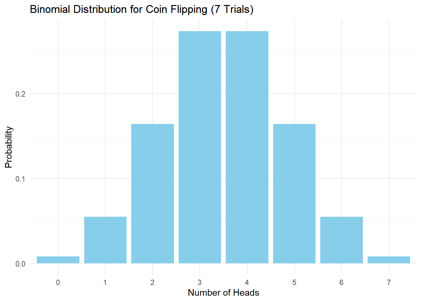
The Probability Mass Function (PMF) is specifically designed for discrete random variables, where the set of possible values the variable can take is countable and distinct. It provides the probability distribution for each of these specific values.
For continuous random variables, where the set of possible values is uncountably infinite (such as all real numbers within a range), we use a Probability Density Function (PDF) instead of a PMF. The PDF gives the probability density at each point within the range of the variable’s values, and the probability of obtaining a specific value in a continuous distribution is calculated using integration over a range, rather than summing probabilities as in a PMF.
For instance, consider a continuous variable like the height of individuals in a population. It’s a continuous range, and the likelihood of obtaining an exact value (e.g., exactly 175 cm) from a continuous distribution is infinitesimally small due to the infinite number of potential values.
Therefore, while PMF is suitable for discrete variables like rolling a die or counting occurrences, continuous variables are typically analyzed using probability density functions (PDFs) or cumulative distribution functions (CDFs) that describe the probability of a variable falling within a certain range rather than taking on a specific value.
In summary, the PMF is not applicable to continuous variables due to their infinitely uncountable nature; instead, continuous variables are described using PDFs or CDFs.
Statistics and Data Analysis: Probability forms the foundation of statistics, which involves collecting, analyzing, interpreting, and presenting data. Probability distributions and concepts like sampling, hypothesis testing, and confidence intervals are essential for making informed decisions based on data.
Science and Engineering: Probability is used extensively in scientific research and engineering to model and analyze complex systems. It plays a crucial role in fields like physics, chemistry, biology, and environmental science, helping researchers predict outcomes and understand phenomena subject to random variations.
Finance and Economics: Probability models are integral to risk assessment, portfolio management, and pricing of financial derivatives. In economics, probability helps analyze market trends, forecast economic indicators, and evaluate the impact of policies.
Machine Learning and Artificial Intelligence: In AI and machine learning, probability is used to model uncertainty and make predictions. Bayesian networks, hidden Markov models, and probabilistic graphical models are used to develop intelligent systems that can make decisions in uncertain environments.
Medicine and Healthcare: Probability is used in medical diagnostics, epidemiology, and clinical trials. It helps assess the effectiveness of treatments, predict disease outcomes, and estimate the spread of diseases.
Information Theory and Communication: Probability is central to information theory, which underlies modern communication systems. It’s used to quantify information content, design error-correcting codes, and optimize data compression algorithms.
Social Sciences: Probability is used to model and analyze social phenomena, such as public opinion polling, demographic trends, and decision-making processes. It’s also used in psychology to study cognitive processes and behavior.
Environmental Science: Probability models are used to predict natural events like weather patterns, seismic activities, and ecological changes. These models aid in disaster preparedness and resource management.
Quality Control and Manufacturing: Probability and statistics are crucial in quality control processes for ensuring consistent product quality. They help identify defects, maintain production standards, and improve manufacturing processes.
Gaming and Gambling: Probability is foundational to games of chance and gambling. Understanding probabilities can help players make informed decisions and develop strategies in games like poker, blackjack, and roulette.
Law and Criminal Justice: Probability is used in forensic science to analyze evidence, estimate the likelihood of a certain event occurring, and assess the reliability of eyewitness testimony.
Risk Management and Insurance: Probability is used to assess risks and set insurance premiums. It helps insurers quantify potential losses and design policies that balance risk and coverage.
In essence, probability provides a systematic framework for understanding uncertainty and making informed decisions in various fields. Its applications are far-reaching and play a vital role in shaping our understanding of the world around us.
Here, I’m offering a straightforward script to compute the ratio between two numerical variables and generate a printed output with the result. In the context of R, we employ the paste() function to combine strings along with variable values. This bears similarity to the functionality of printf(), which is used in various other programming languages.↩︎
In the preceding script, I introduced another useful function in R called round(). This function takes two arguments: the first being a floating-point number, and the second being the number of decimal places to which I intend to round off the number.↩︎
Author: OpenAI. (2023, October 31). “Definition of Probability Distribution” (Version 1). ChatGPT. https://www.openai.com↩︎
also can be calculated using combinatorics, omitting with purpose on this book, but take a look on the class of MAT 207, is fun! ^^↩︎
Author: OpenAI. (2023, October 31). “Definition and Requirements for a Binomial Distribution” (Version 1). ChatGPT. https://www.openai.com↩︎