In this appendix, we will use a publicly available dataset from our research group on fitbit at ORU, analyzing it without referencing the paper published by our group in 2019.
C.1 Context of the Data
This dataset is from the most cited article by our group, referenced 21 times as of June 19, 2024.1
Reference: Broaddus, Allie; Jaquis, Brandon; Jones, Colt; Jost, Scarlet; Lang, Andrew; Li, Ailin; et al. (2018). Dataset: Fitbits, field-tests, and grades. The effects of a healthy and physically active lifestyle on the academic performance of first-year college students. figshare. Dataset. https://doi.org/10.6084/m9.figshare.7218497.v1
C.1.1 Data Collection
The data were collected during the Fall semester of 2017 from 581 freshmen enrolled at Oral Roberts University in a class titled “Introduction to Whole Person Education.” This course includes a mandatory health and physical exercise component, consisting of:
Steps and Active Minutes goals
A 1-mile field test
A lifestyle assessment survey
Students utilized Fitbits to track their steps and active minutes, which were synced with the course gradebook. The students’ semester grade point averages (GPAs) were recorded at the end of the semester. To ensure confidentiality, the dataset was de-identified after the grades were retrieved and stored.
C.2 Loading the dataset
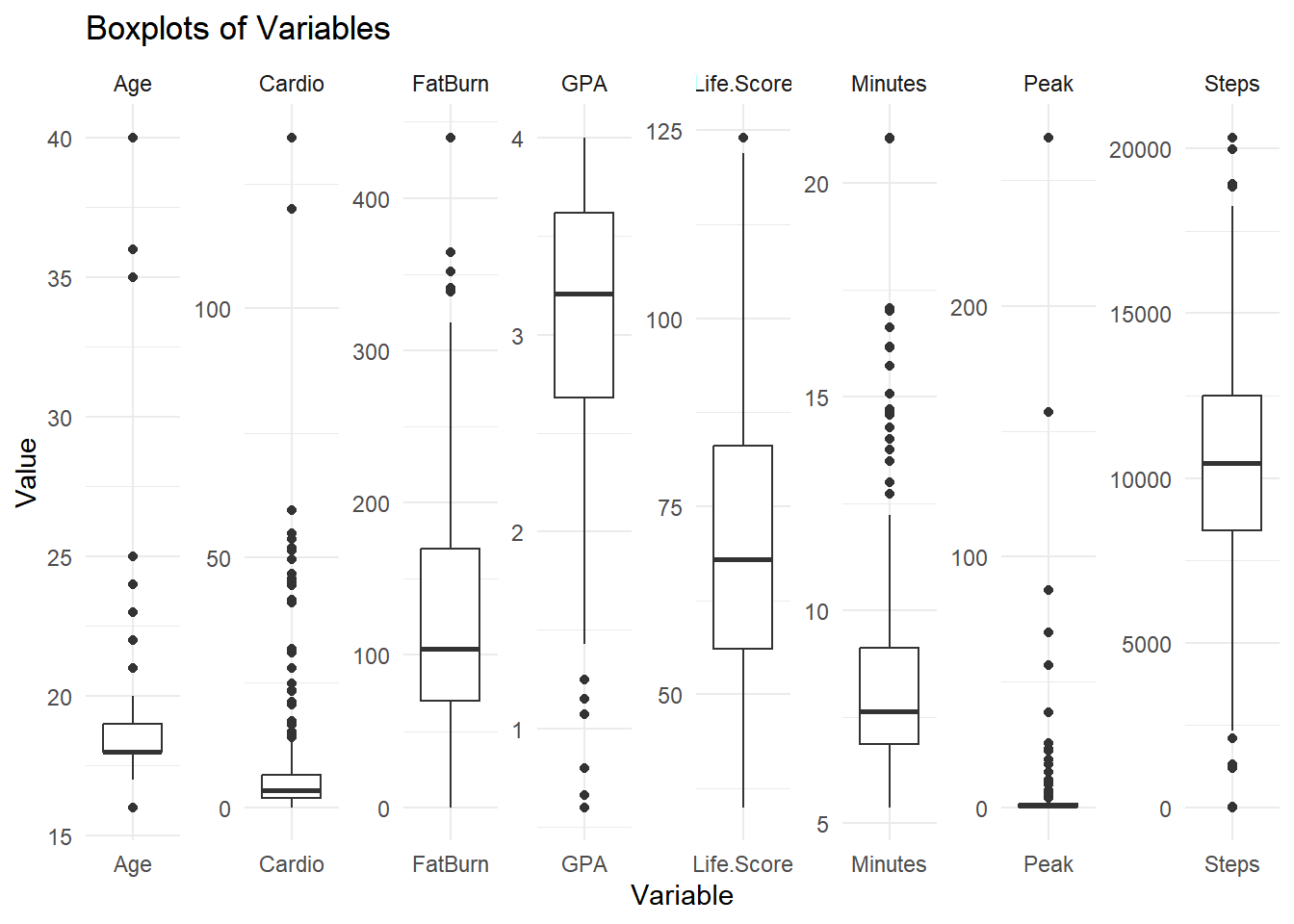
df <-read.csv("FitbitsAndGradesData_Fall2017.csv")str(df) # quick overview of the data
      Key            Steps            Peak            Cardio
 Min.   :  3.0   Min.   :    9   Min.   :  0.00   Min.   :  0.000
 1st Qu.:138.0   1st Qu.: 8399   1st Qu.:  0.20   1st Qu.:  1.830
 Median :282.0   Median :10455   Median :  0.58   Median :  3.340
 Mean   :282.5   Mean   :10425   Mean   :  4.54   Mean   :  8.308
 3rd Qu.:425.0   3rd Qu.:12497   3rd Qu.:  1.54   3rd Qu.:  6.570
 Max.   :581.0   Max.   :20331   Max.   :267.10   Max.   :134.200
    FatBurn            Mode           Minutes           Gender       Age
 Min.   :  0.01   Min.   :0.0000   Min.   : 5.380   Min.   :0   Min.   :16.00
 1st Qu.: 69.84   1st Qu.:1.0000   1st Qu.: 6.850   1st Qu.:0   1st Qu.:18.00
 Median :104.09   Median :1.0000   Median : 7.630   Median :0   Median :18.00
 Mean   :122.16   Mean   :0.9114   Mean   : 8.586   Mean   :0   Mean   :18.85
 3rd Qu.:169.65   3rd Qu.:1.0000   3rd Qu.: 9.120   3rd Qu.:0   3rd Qu.:19.00
 Max.   :439.58   Max.   :1.0000   Max.   :21.070   Max.   :0   Max.   :40.00
      GPA          Life.Score
 Min.   :0.600   Min.   : 35.00
 1st Qu.:2.680   1st Qu.: 56.00
 Median :3.210   Median : 68.00
 Mean   :3.054   Mean   : 69.98
 3rd Qu.:3.620   3rd Qu.: 83.00
 Max.   :4.000   Max.   :124.00
      Key            Steps            Peak            Cardio
 Min.   :  1.0   Min.   :    0   Min.   : 0.000   Min.   :  0.000
 1st Qu.:156.8   1st Qu.: 8771   1st Qu.: 0.385   1st Qu.:  3.098
 Median :305.5   Median :10187   Median : 0.945   Median :  5.780
 Mean   :296.8   Mean   :10094   Mean   : 1.708   Mean   :  9.490
 3rd Qu.:444.2   3rd Qu.:11790   3rd Qu.: 2.152   3rd Qu.:  9.852
 Max.   :580.0   Max.   :18673   Max.   :36.180   Max.   :180.650
    FatBurn            Mode           Minutes          Gender       Age
 Min.   :  0.00   Min.   :0.0000   Min.   : 5.58   Min.   :1   Min.   :16.00
 1st Qu.: 98.27   1st Qu.:1.0000   1st Qu.: 8.91   1st Qu.:1   1st Qu.:18.00
 Median :136.62   Median :1.0000   Median :10.79   Median :1   Median :18.00
 Mean   :167.03   Mean   :0.8169   Mean   :11.25   Mean   :1   Mean   :18.46
 3rd Qu.:214.15   3rd Qu.:1.0000   3rd Qu.:13.21   3rd Qu.:1   3rd Qu.:19.00
 Max.   :729.67   Max.   :1.0000   Max.   :19.10   Max.   :1   Max.   :25.00
      GPA          Life.Score
 Min.   :0.000   Min.   : 35.00
 1st Qu.:2.920   1st Qu.: 58.00
 Median :3.500   Median : 70.00
 Mean   :3.278   Mean   : 71.91
 3rd Qu.:3.820   3rd Qu.: 83.00
 Max.   :4.000   Max.   :130.00
C.4 Analysis from summary of statistics
C.4.1 Key Observations:
Steps:
Males show a slightly higher mean and median steps compared to females, indicating a higher average step count. However, the broader range for males suggests greater variability and possibly the presence of subgroups within the male population.
Peak and Cardio:
Males have a higher mean peak value and a much larger maximum value, indicating more intense peaks in activity levels. Cardio values are relatively similar in means, but females have a higher maximum cardio value.
FatBurn:
Females have a higher mean and maximum fat burn values, suggesting that on average, they spend more time in the fat burn zone compared to males.
Minutes:
The Minutes variable contains the recorded times for a required field test. Females have higher mean and median minutes, suggesting they need more time to complete the field test.
Age:
Both groups have a similar age range, but males have a slightly higher mean age.
GPA:
Females have a higher mean and median GPA, indicating better academic performance on average compared to males.
Life.Score:
Females have a higher mean life score, suggesting a lower overall quality of life or well-being compared to males.
C.4.2 Conclusion:
The summary and visual statistics reveal that males tend to have more variability in their physical activity levels, with a wider range of steps and peaks, potentially indicating the presence of distinct subgroups within the male population. Females, on the other hand, exhibit more consistent activity levels with higher fat burn and overall minutes spent in activity. Academically, females outperform males on average, as indicated by higher GPA scores. Both groups show a similar range in age and life scores, with females having slightly higher life scores on average.
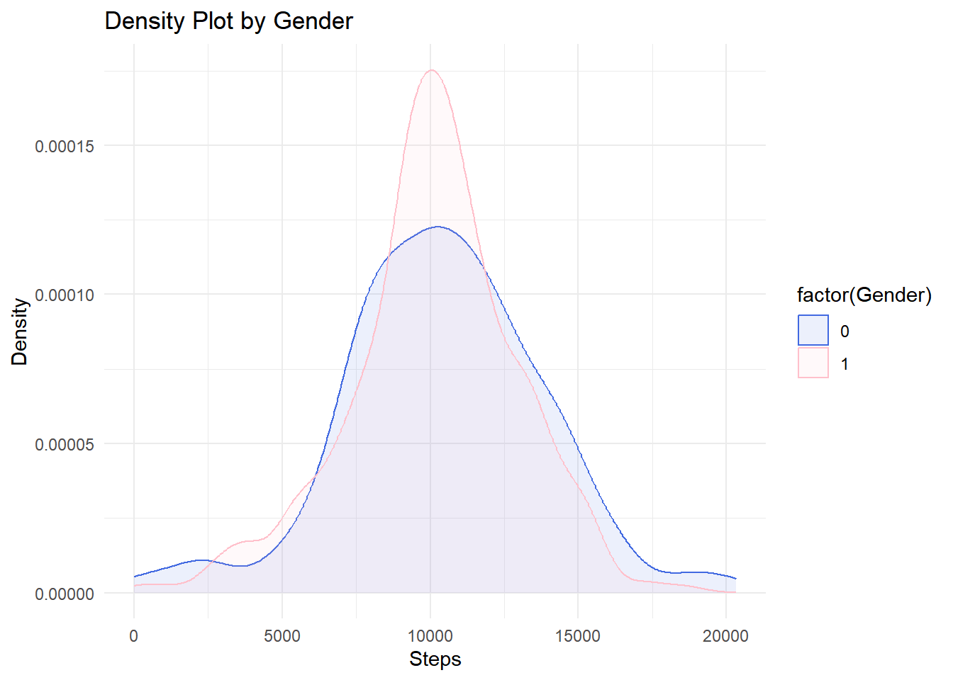
C.5 Distribution of Steps per gender
The density plot displays the distribution of steps taken by two groups based on gender. Several key observations can be made from the plot:
Broader Distribution for Males (0):
The distribution for males (blue curve) is broader, indicating greater variability in the number of steps taken. This suggests that there might be at least two subgroups within the male participants. One subgroup could be more active, averaging a higher number of steps per week, while another subgroup could be less active.
Uniform Distribution for Females (1):
The distribution for females (pink curve) is narrower and more symmetric compared to the males. This indicates that the number of steps taken by female participants is more consistent across the group. The symmetry suggests a more homogeneous activity level among females.
Shoulder in Female Distribution:
A noticeable shoulder on the right side of the female distribution curve indicates a small subset of females who are more active than the average. This subgroup, while not as large as the main peak, suggests that there are some females who take a significantly higher number of steps.
C.5.1 Analysis from density distribution visualization:
The density plot highlights distinct differences in the activity patterns between males and females. Males exhibit a wider range of activity levels, possibly due to the presence of distinct subgroups with different activity levels. In contrast, females show a more uniform activity pattern, though with a small subset displaying higher activity levels. Understanding these differences could be valuable for tailoring health and fitness programs to better meet the needs of each gender group.
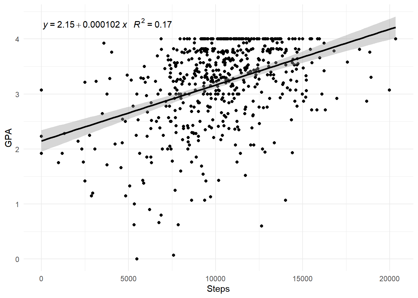
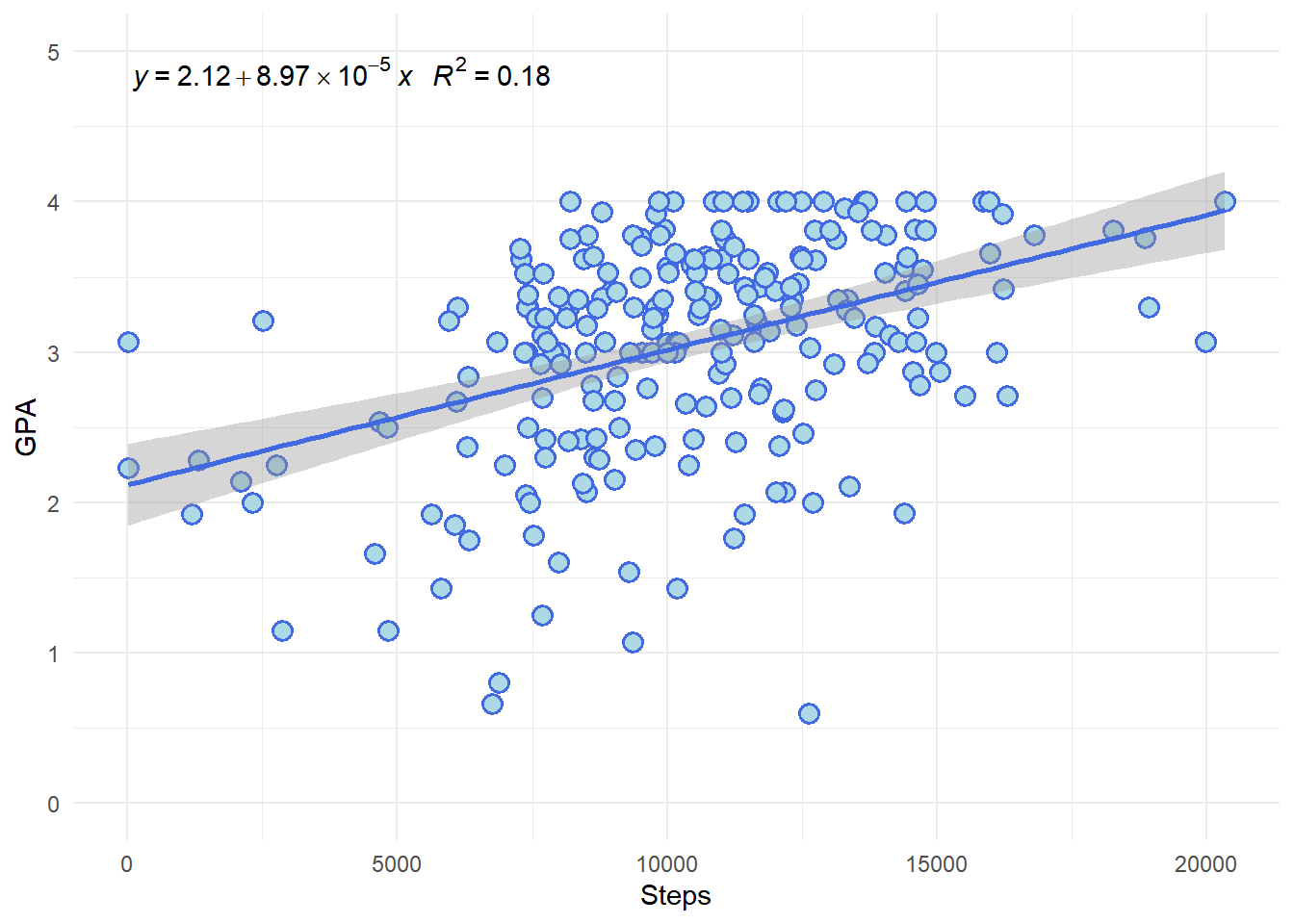
C.6 Analysis of GPA vs. Steps
To investigate the impact of physical activity on overall academic performance, we performed a linear regression analysis using the number of steps as the predictor variable and GPA as the response variable. Below is the summary of the regression model and the corresponding scatter plot with the regression line.
C.6.1 Scatter Plot with Regression Line
The scatter plot shows the relationship between the number of steps taken and the GPA of the students. A regression line has been added to illustrate the trend.
Residual standard error: 0.6914 on 579 degrees of freedom Multiple R-squared: 0.1689 Adjusted R-squared: 0.1675 F-statistic: 117.7 on 1 and 579 DF p-value: < 2.2e-16
C.6.3 Interpretation of Results
Intercept (Estimate = 2.148): The intercept represents the average GPA when the number of steps is zero. This value is statistically significant (p < 2e-16).
Slope (Estimate = 0.0001015): The slope indicates that for every additional 10,000 steps, the GPA increases by approximately 1.015. This relationship is statistically significant (p < 2e-16).
R-squared (0.1689): This value indicates that approximately 16.89% of the variability in GPA can be explained by the number of steps taken. While this suggests a positive correlation, it also indicates that there are other factors influencing GPA that are not accounted for in this model.
C.6.4 Conclusion
The regression analysis suggests a statistically significant positive relationship between physical activity (measured by steps) and academic performance (GPA). However, the relatively low R-squared value indicates that other factors also play a significant role in determining GPA. Further research could include additional variables to build a more comprehensive model.
Call:
lm(formula = GPA ~ ., data = df)

Residuals:
    Min      1Q  Median      3Q     Max
-3.0274 -0.3591  0.1385  0.4772  1.4102

Coefficients: (1 not defined because of singularities)
                  Estimate Std. Error t value Pr(>|t|)
(Intercept)      2.318e+00  4.170e-01   5.557 4.21e-08 ***
Key             -5.512e-05  1.687e-04  -0.327   0.7439
Steps            9.312e-05  1.016e-05   9.166  < 2e-16 ***
Peak            -1.919e-03  2.135e-03  -0.899   0.3690
Cardio           1.923e-03  2.066e-03   0.931   0.3523
FatBurn          1.519e-04  3.639e-04   0.417   0.6765
Mode             4.535e-02  1.101e-01   0.412   0.6807
Minutes         -2.668e-02  1.425e-02  -1.873   0.0616 .
Gender           3.250e-01  6.586e-02   4.934 1.06e-06 ***
Age              7.757e-03  1.702e-02   0.456   0.6486
Life.Score      -2.899e-03  1.586e-03  -1.828   0.0681 .
GenderLabelMale         NA         NA      NA       NA
---
Signif. codes:  0 '***' 0.001 '**' 0.01 '*' 0.05 '.' 0.1 ' ' 1

Residual standard error: 0.6758 on 570 degrees of freedom
Multiple R-squared:  0.2183,    Adjusted R-squared:  0.2046
F-statistic: 15.92 on 10 and 570 DF,  p-value: < 2.2e-16
C.9 Analysis
C.9.1 Main Results
The linear regression analysis was performed to predict GPA based on various predictor variables. Here are the key findings from the analysis:
Intercept: The intercept of the model is 2.318, which is statistically significant (p < 0.001).
Steps: The number of Steps taken has a positive and highly significant effect on GPA (estimate = 0.00009312, p < 0.001).
Peak: The coefficient for Peak is -0.001919, but it is not statistically significant (p = 0.3690).
Cardio: The Cardio variable has a positive but not statistically significant effect on GPA (estimate = 0.001923, p = 0.3523).
FatBurn: The coefficient for FatBurn is 0.0001519, but it is not statistically significant (p = 0.6765).
Mode: The effect of Mode on GPA is positive but not statistically significant (estimate = 0.04535, p = 0.6807).
Minutes: The Minutes variable has a negative effect on GPA, with a marginal level of significance (estimate = -0.02668, p = 0.0616).
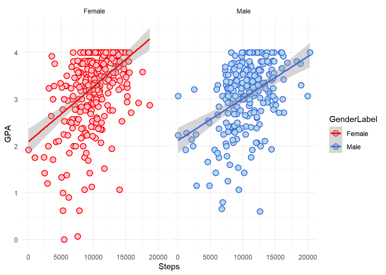
Gender: Being male (Gender = 0) has a positive and highly significant effect on GPA (estimate = 0.3250, p < 0.001).
Age: The effect of Age on GPA is positive but not statistically significant (estimate = 0.007757, p = 0.6486).
Life.Score: The Life.Score has a negative effect on GPA with a marginal level of significance (estimate = -0.002899, p = 0.0681).
C.9.2 Model Summary
Residual standard error: 0.6758 on 570 degrees of freedom.
Multiple R-squared: 0.2183, indicating that approximately 21.83% of the variability in GPA is explained by the model.
Adjusted R-squared: 0.2046, which adjusts the R-squared value based on the number of predictors in the model.
F-statistic: 15.92 on 10 and 570 DF, with a p-value < 2.2e-16, indicating that the overall model is statistically significant.
C.9.3 Conclusion
The linear regression analysis shows that Steps and Gender (with males having higher GPAs) are significant predictors of GPA. Other variables such as Minutes and Life.Score show marginal significance, while the rest of the variables do not significantly contribute to the model. Despite the statistical significance of some predictors, the model explains only a modest proportion of the variability in GPA (approximately 21.83%), suggesting that other factors not included in the model may also play a substantial role in determining GPA.
C.10 Controlling by gender
C.10.1 Searching for best model for males
model_m <-lm(GPA~.,data=df_m)summary(model_m)
Call:
lm(formula = GPA ~ ., data = df_m)

Residuals:
     Min       1Q   Median       3Q      Max
-2.86289 -0.35140  0.09225  0.43291  1.47888

Coefficients: (1 not defined because of singularities)
              Estimate Std. Error t value Pr(>|t|)
(Intercept)  3.714e+00  5.792e-01   6.412 8.22e-10 ***
Key          2.323e-04  2.529e-04   0.918  0.35936
Steps        7.309e-05  1.334e-05   5.479 1.13e-07 ***
Peak        -2.402e-03  2.138e-03  -1.123  0.26247
Cardio       1.076e-03  3.294e-03   0.327  0.74415
FatBurn      1.377e-03  6.822e-04   2.018  0.04477 *
Mode        -6.378e-01  2.433e-01  -2.622  0.00934 **
Minutes     -9.250e-02  2.446e-02  -3.781  0.00020 ***
Gender              NA         NA      NA       NA
Age         -3.577e-03  1.833e-02  -0.195  0.84542
Life.Score  -3.010e-03  2.356e-03  -1.278  0.20269
---
Signif. codes:  0 '***' 0.001 '**' 0.01 '*' 0.05 '.' 0.1 ' ' 1

Residual standard error: 0.6342 on 227 degrees of freedom
Multiple R-squared:  0.2542,    Adjusted R-squared:  0.2246
F-statistic: 8.597 on 9 and 227 DF,  p-value: 4.536e-11
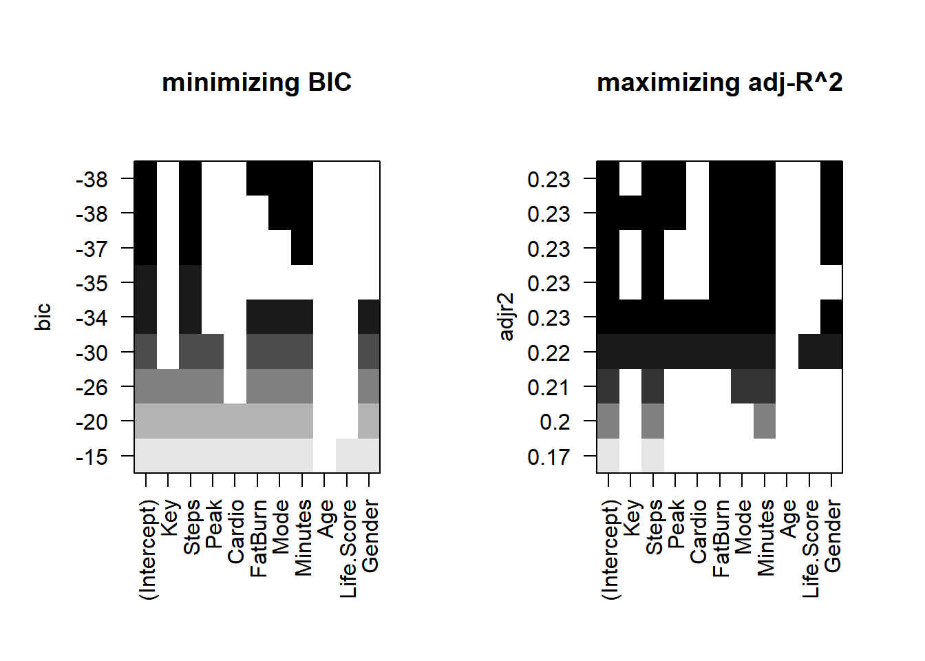
library(leaps)a <-regsubsets(GPA~.,data=df_m)
Warning in leaps.setup(x, y, wt = wt, nbest = nbest, nvmax = nvmax, force.in =
force.in, : 1 linear dependencies found
When selecting the best model, we consider various statistical metrics and criteria, such as the adjusted R-squared, the p-value of the F-statistic, and the Bayesian Information Criterion (BIC). Let’s compare the two models in detail:
C.10.3.1 Model 1:
Formula:GPA ~ Steps + FatBurn + Mode + Minutes
Residual standard error: 0.6323 on 232 degrees of freedom
Residual standard error: 0.6314 on 230 degrees of freedom
Multiple R-squared: 0.251
Adjusted R-squared: 0.2314
F-statistic: 12.84 on 6 and 230 DF
p-value of F-statistic: 1.663e-12
Significant predictors:
Steps (p-value: 8.72e-08 ***)
FatBurn (p-value: 0.011782 *)
Mode (p-value: 0.010486 *)
Minutes (p-value: 0.000151 ***)
Peak and Life.Score were not significant.
C.10.4 Model Comparison and Selection
Adjusted R-squared: Model 2 has a slightly higher adjusted R-squared (0.2314) compared to Model 1 (0.2291), indicating a slightly better fit.
p-value of F-statistic: Model 1 has a slightly lower p-value (3.122e-13) compared to Model 2 (1.663e-12), suggesting that Model 1 has a marginally better overall significance.
Residual Standard Error: Model 2 has a slightly lower residual standard error (0.6314) compared to Model 1 (0.6323), indicating that Model 2’s predictions are marginally closer to the actual values.
Significant Predictors: Both models have Steps, FatBurn, Mode, and Minutes as significant predictors. However, Model 2 introduces Peak and Life.Score, which are not significant.
C.10.5 Conclusion
Despite Model 2 having a slightly higher adjusted R-squared, the introduction of non-significant predictors (Peak and Life.Score) does not substantially improve the model. Given that both models are quite similar in performance, I choose Model 1 for its simplicity and slightly better p-value of the F-statistic.
Reason: Model 1 is chosen because it has a comparable adjusted R-squared, a lower p-value of the F-statistic, and it avoids the inclusion of non-significant predictors, maintaining model simplicity and interpretability.
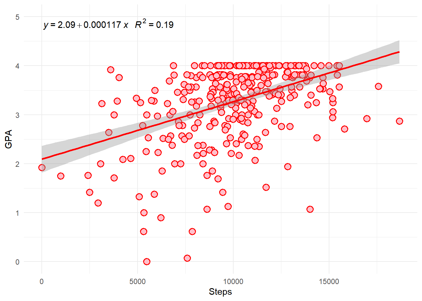
C.10.6 Searching for best model for females
model_f <-lm(GPA~.,data=df_f)summary(model_f)
Call:
lm(formula = GPA ~ ., data = df_f)

Residuals:
    Min      1Q  Median      3Q     Max
-2.8958 -0.3379  0.1617  0.5011  1.4613

Coefficients: (1 not defined because of singularities)
              Estimate Std. Error t value Pr(>|t|)
(Intercept)  1.991e+00  7.948e-01   2.504   0.0127 *
Key         -2.590e-04  2.239e-04  -1.157   0.2482
Steps        1.126e-04  1.538e-05   7.319 1.87e-12 ***
Peak         3.035e-02  1.671e-02   1.816   0.0703 .
Cardio      -1.168e-03  3.110e-03  -0.376   0.7074
FatBurn     -2.412e-04  4.386e-04  -0.550   0.5828
Mode         1.779e-01  1.260e-01   1.411   0.1591
Minutes      5.754e-03  1.930e-02   0.298   0.7658
Gender              NA         NA      NA       NA
Age          1.056e-02  3.802e-02   0.278   0.7813
Life.Score  -2.467e-03  2.136e-03  -1.155   0.2489
---
Signif. codes:  0 '***' 0.001 '**' 0.01 '*' 0.05 '.' 0.1 ' ' 1

Residual standard error: 0.6922 on 334 degrees of freedom
Multiple R-squared:  0.2139,    Adjusted R-squared:  0.1927
F-statistic:  10.1 on 9 and 334 DF,  p-value: 9.319e-14
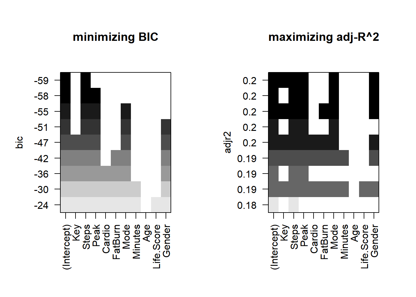
library(leaps)a <-regsubsets(GPA~.,data=df_f)
Warning in leaps.setup(x, y, wt = wt, nbest = nbest, nvmax = nvmax, force.in =
force.in, : 1 linear dependencies found
Call:
lm(formula = GPA ~ Steps, data = df_f)

Residuals:
    Min      1Q  Median      3Q     Max
-2.9148 -0.3437  0.1579  0.4991  1.4046

Coefficients:
             Estimate Std. Error t value Pr(>|t|)
(Intercept) 2.093e+00  1.389e-01  15.075   <2e-16 ***
Steps       1.174e-04  1.325e-05   8.862   <2e-16 ***
---
Signif. codes:  0 '***' 0.001 '**' 0.01 '*' 0.05 '.' 0.1 ' ' 1

Residual standard error: 0.6958 on 342 degrees of freedom
Multiple R-squared:  0.1868,    Adjusted R-squared:  0.1844
F-statistic: 78.54 on 1 and 342 DF,  p-value: < 2.2e-16
C.10.7.2 Model 4: max(adjr2) for only females
Call:
lm(formula = GPA ~ Steps + Peak + Mode + Life.Score, data = df_f)

Residuals:
    Min      1Q  Median      3Q     Max
-2.9738 -0.3251  0.1666  0.4980  1.4064

Coefficients:
              Estimate Std. Error t value Pr(>|t|)
(Intercept)  2.194e+00  2.149e-01  10.210  < 2e-16 ***
Steps        1.093e-04  1.342e-05   8.143 7.47e-15 ***
Peak         2.413e-02  1.308e-02   1.845   0.0659 .
Mode         1.680e-01  9.798e-02   1.715   0.0872 .
Life.Score  -2.745e-03  2.010e-03  -1.366   0.1730
---
Signif. codes:  0 '***' 0.001 '**' 0.01 '*' 0.05 '.' 0.1 ' ' 1

Residual standard error: 0.6893 on 339 degrees of freedom
Multiple R-squared:  0.2088,    Adjusted R-squared:  0.1994
F-statistic: 22.36 on 4 and 339 DF,  p-value: < 2.2e-16
C.10.8 Best Model Rationale for Females
C.10.8.1 Model 3: Minimizing BIC
Formula:GPA ~ Steps
Residual standard error: 0.6958 on 342 degrees of freedom
Multiple R-squared: 0.1868
Adjusted R-squared: 0.1844
F-statistic: 78.54 on 1 and 342 DF
p-value of F-statistic: < 2.2e-16
Significant predictors:
Steps (p-value: <2e-16 ***)
C.10.8.2 Model 4: Maximizing Adjusted R-squared
Formula:GPA ~ Steps + Peak + Mode + Life.Score
Residual standard error: 0.6893 on 339 degrees of freedom
Multiple R-squared: 0.2088
Adjusted R-squared: 0.1994
F-statistic: 22.36 on 4 and 339 DF
p-value of F-statistic: < 2.2e-16
Significant predictors:
Steps (p-value: 7.47e-15 ***)
Peak (p-value: 0.0659 .)
Mode (p-value: 0.0872 .)
Life.Score (p-value: 0.1730)
C.10.9 Model Comparison and Selection for Females
Adjusted R-squared: Model 4 has a higher adjusted R-squared (0.1994) compared to Model 3 (0.1844), indicating that Model 4 explains more variability in GPA for females.
p-value of F-statistic: Both models have highly significant p-values, suggesting that both models are statistically significant overall.
Residual Standard Error: Model 4 has a slightly lower residual standard error (0.6893) compared to Model 3 (0.6958), indicating that Model 4’s predictions are marginally closer to the actual values.
Significant Predictors:
In Model 3, Steps is a highly significant predictor.
In Model 4, Steps remains highly significant, while Peak and Mode show marginal significance, and Life.Score is not significant.
C.10.10 Conclusion
While Model 4 has a higher adjusted R-squared and a slightly lower residual standard error, it includes predictors (Peak, Mode, and Life.Score) that are not strongly significant. Given the trade-off between model complexity and statistical significance of predictors, Model 3 is preferred for its simplicity and the high significance of the Steps predictor.
Chosen Model for Females:GPA ~ Steps
Reason: Model 3 is chosen because it is simpler and includes only the highly significant predictor, Steps. This simplicity and significance make it a more interpretable and reliable model for predicting GPA in females.
C.11 DrV’s Recommendations
C.11.1 Explanation and Recommendations:
Males:
Best Model:GPA ~ Steps + FatBurn + Mode + Minutes
Interpretation: This model indicates that GPA is influenced by a combination of steps taken, fat burned, the mode of activity (running or walking), and the minutes spent to complete the field test.
Recommendation: Males should engage in higher intensity activities to improve GPA. Suggested activities include:
Running or brisk walking: To increase both the number of steps and the amount of fat burned.
Structured exercise routines: Spending more time on these activities to maximize benefits.
Females:
Best Model:GPA ~ Steps
Interpretation: This model shows that GPA is primarily influenced by the number of steps taken.
Recommendation: Females can achieve positive results with low-intensity activities. Suggested activities include:
Daily walking: A simple and effective way to increase the number of steps and enhance GPA.
C.11.2 Summary:
For Males: A more intensive exercise routine, including activities like running or other cardiovascular exercises, is recommended. These activities help in burning more fat and increasing the time spent exercising, which positively impacts GPA.
For Females: Low-intensity activities like daily walking are sufficient and beneficial for improving GPA. This approach leverages the simplicity and effectiveness of walking to achieve positive academic outcomes.
These recommendations align with physiological differences between males and females, suggesting that males may benefit more from higher intensity activities, while females can achieve positive outcomes with moderate, consistent physical activity.