It would be remiss to delve into a book about probability and statistics without addressing the pivotal role they play in the realm of machine learning. Neglecting this essential application within mathematics and computing would do injustice to its significance. In conclusion, this chapter aims to bridge this gap by delving into crucial modeling techniques and demonstrating how data correlations are harnessed to make predictions. The discussion will encompass pivotal methods like Linear Models, Binomial Models, and Random Forest Modeling, serving as a culmination of our exploration. This chapter effectively puts the entire spectrum of knowledge into action, bringing the concepts to life.
7.1 Linear Modeling
Linear modeling is a fundamental statistical method used to understand and predict the relationship between a dependent variable and one or more independent variables. It assumes a linear relationship between the variables, where changes in the independent variables are associated with changes in the dependent variable by a constant factor.
R offers robust tools and libraries to perform linear modeling. The lm() function is commonly used to create linear models, enabling researchers, data scientists, and analysts to explore relationships between variables, make predictions, and draw insights from data.
7.1.1 Key Concepts in Linear Modeling:
Dependent Variable (Response Variable): The variable being predicted or explained by the model.
Independent Variables (Predictor Variables): The variables used to predict or explain changes in the dependent variable. In multiple linear regression, there are more than one independent variable.
Coefficients: Represent the estimated relationship between the independent variables and the dependent variable. They indicate how much the dependent variable changes when the independent variable changes by one unit, assuming other variables are held constant.
Residuals: Differences between the observed values and the values predicted by the model. Residual analysis helps evaluate how well the model fits the data.
7.1.2 Steps in Linear Modeling using R:
Data Preparation: Load and explore the dataset to understand the variables and their distributions, checking for missing values and outliers.
Model Building: Use the lm() function to build a linear regression model. Specify the formula with the dependent variable and independent variables.
Model Evaluation: Examine the model summary using summary() to assess the coefficients, p-values, R-squared value, and other statistical measures. Interpret the significance of predictors and overall model fit.
Model Diagnostics: Validate assumptions such as linearity, normality of residuals, constant variance (homoscedasticity), and independence of residuals. Plotting residuals and performing diagnostic tests are common practices.
Prediction and Inference: Use the model to make predictions on new data and infer relationships between variables.
7.1.3 Conclusion:
Linear modeling in R provides a systematic approach to understand the relationships between variables, enabling data-driven decision-making, hypothesis testing, and predictive analytics. By leveraging R’s functionalities, analysts can build, assess, and interpret linear models to gain insights into their data and make informed conclusions.
How can the mtcars dataset be explored and utilized to perform multiple linear regression for predicting mpg (miles per gallon) based on hp (horsepower), wt (weight), and disp (displacement)? Furthermore, what insights can be derived from the summary output of the regression model regarding the relationships between the predictor variables and the target variable (mpg)?”
EXPLORATORY DATA ANALYSIS (EDA)
7.1.4 Step 1: Load the dataset and explore it
# Load the 'mtcars' datasetdata(mtcars)# View the structure of the datasetstr(mtcars)
# Summary statistics of the datasetsummary(mtcars)
      mpg             cyl             disp             hp
 Min.   :10.40   Min.   :4.000   Min.   : 71.1   Min.   : 52.0
 1st Qu.:15.43   1st Qu.:4.000   1st Qu.:120.8   1st Qu.: 96.5
 Median :19.20   Median :6.000   Median :196.3   Median :123.0
 Mean   :20.09   Mean   :6.188   Mean   :230.7   Mean   :146.7
 3rd Qu.:22.80   3rd Qu.:8.000   3rd Qu.:326.0   3rd Qu.:180.0
 Max.   :33.90   Max.   :8.000   Max.   :472.0   Max.   :335.0
      drat             wt             qsec             vs
 Min.   :2.760   Min.   :1.513   Min.   :14.50   Min.   :0.0000
 1st Qu.:3.080   1st Qu.:2.581   1st Qu.:16.89   1st Qu.:0.0000
 Median :3.695   Median :3.325   Median :17.71   Median :0.0000
 Mean   :3.597   Mean   :3.217   Mean   :17.85   Mean   :0.4375
 3rd Qu.:3.920   3rd Qu.:3.610   3rd Qu.:18.90   3rd Qu.:1.0000
 Max.   :4.930   Max.   :5.424   Max.   :22.90   Max.   :1.0000
       am              gear            carb
 Min.   :0.0000   Min.   :3.000   Min.   :1.000
 1st Qu.:0.0000   1st Qu.:3.000   1st Qu.:2.000
 Median :0.0000   Median :4.000   Median :2.000
 Mean   :0.4062   Mean   :3.688   Mean   :2.812
 3rd Qu.:1.0000   3rd Qu.:4.000   3rd Qu.:4.000
 Max.   :1.0000   Max.   :5.000   Max.   :8.000
Load the ‘mtcars’ dataset: The data(mtcars) command loads the built-in ‘mtcars’ dataset in R. This dataset contains data on various car models and their characteristics, such as miles per gallon (mpg), horsepower (hp), weight (wt), and other attributes.
View the structure of the dataset: The str(mtcars) command displays the structure of the ‘mtcars’ dataset. It provides information about the variables (columns), their data types, and the first few values. This function helps to understand the composition and organization of the dataset.
View the first few rows of the dataset: The head(mtcars) command shows the first few rows of the ‘mtcars’ dataset. By default, it displays the first six rows, providing a glimpse of the data’s contents, including the variables and their values.
Summary statistics of the dataset: The summary(mtcars) command generates summary statistics for each numerical variable in the ‘mtcars’ dataset. For each numeric variable, it presents descriptive statistics such as minimum, 1st quartile, median, mean, 3rd quartile, maximum, and sometimes additional information like standard deviation.
7.1.5 Step 2: Perform multiple linear regression
Let’s say we want to predict mpg (miles per gallon) using hp (horsepower), wt (weight), and disp (displacement).
# Fit the multiple linear regression modelmodel <-lm(mpg ~ hp + wt + disp, data = mtcars)# View the summary of the modelsummary(model)
Call:
lm(formula = mpg ~ hp + wt + disp, data = mtcars)

Residuals:
   Min     1Q Median     3Q    Max
-3.891 -1.640 -0.172  1.061  5.861

Coefficients:
             Estimate Std. Error t value Pr(>|t|)
(Intercept) 37.105505   2.110815  17.579  < 2e-16 ***
hp          -0.031157   0.011436  -2.724  0.01097 *
wt          -3.800891   1.066191  -3.565  0.00133 **
disp        -0.000937   0.010350  -0.091  0.92851
---
Signif. codes:  0 '***' 0.001 '**' 0.01 '*' 0.05 '.' 0.1 ' ' 1

Residual standard error: 2.639 on 28 degrees of freedom
Multiple R-squared:  0.8268,    Adjusted R-squared:  0.8083
F-statistic: 44.57 on 3 and 28 DF,  p-value: 8.65e-11
Fitting a Multiple Linear Regression Model: The line model <- lm(mpg ~ hp + wt + disp, data = mtcars) fits a multiple linear regression model. The formula mpg ~ hp + wt + disp specifies that the target variable (mpg - miles per gallon) is to be predicted based on three predictor variables: hp (horsepower), wt (weight), and disp (displacement). The data = mtcars argument indicates that the data for the model is sourced from the ‘mtcars’ dataset.
Viewing the Summary of the Model: The subsequent line summary(model) displays the summary statistics and information about the fitted linear regression model stored in the model object. The summary includes various details such as coefficients, standard errors, t-values, p-values, R-squared value, adjusted R-squared value, F-statistic, and related statistical measures. These statistics offer insights into the relationships between the predictor variables (hp, wt, disp) and the target variable (mpg) and indicate the overall fit and significance of the model.
7.1.6 Step 3: Interpret the output
The summary() function provides information about the regression model, including coefficients and p-values.
Coefficients: These indicate the estimated coefficients for each predictor variable (hp, wt, disp). They represent the change in mpg for a one-unit change in each predictor variable, holding others constant.
P-values: The p-values associated with each coefficient show the significance of the predictor variables. Lower p-values (usually < 0.05) suggest significant relationships between the predictor and the dependent variable.
In this example:
The intercept is 37.105505.
For every unit increase in hp, mpg decreases by approximately 0.031157 (holding other variables constant).
For every unit increase in wt, mpg decreases by approximately 3.800891 (holding other variables constant).
The coefficient for disp is not statistically significant at the conventional significance level of 0.05 (p-value = 0.92851).
7.1.7 Additional notes:
Ensure the assumptions of linear regression are met.
Interpret the coefficients cautiously, considering the context and nature of the variables.
Visualization and further diagnostics (residual analysis, checking for multicollinearity, etc.) are important for a comprehensive analysis.
7.2 Binomial Models
Binomial models, specifically logistic regression, are widely employed in predictive analytics and machine learning for binary classification tasks. These models are essential when the outcome or dependent variable is binary, representing two possible classes (e.g., yes/no, 0/1, true/false).
In R, logistic regression is a popular statistical method for building binomial models. Unlike linear regression, logistic regression models the probability of a binary outcome by fitting the data to a logistic function, ensuring predictions fall within the range of 0 to 1, representing probabilities.
7.2.1 Key Concepts in Binomial Models:
Binary Outcome: The dependent variable in a classification problem, having two categories.
Logistic Function: The core of logistic regression, mapping input variables to a probability between 0 and 1 using the logistic or sigmoid function.
Logit Transformation: Converts the probability values into a log-odds scale, allowing linear regression to estimate coefficients that represent the change in log-odds for a one-unit change in the predictor variable.
Threshold: A decision threshold is chosen to classify predicted probabilities into discrete classes (e.g., class 0 or class 1).
7.2.2 Steps in Binomial Model Creation using R:
Data Preparation: Explore and preprocess the dataset, including handling missing values, encoding categorical variables, and splitting the data into training and testing sets.
Model Building: Use the glm() (generalized linear model) function in R with a binomial family (e.g., family = "binomial") to fit a logistic regression model. Specify the formula with the dependent variable and predictor variables.
Model Training and Evaluation: Fit the model on the training data, evaluate performance using metrics like accuracy, precision, recall, and ROC curve on the test set.
Model Interpretation: Analyze coefficients and their significance to understand the impact of predictor variables on the binary outcome.
Prediction and Decision Making: Make predictions on new data using the trained model and apply the chosen decision threshold to classify instances.
7.2.3 Conclusion:
Binomial models, especially logistic regression, are powerful tools for binary classification tasks in R. They allow for the estimation of probabilities and offer interpretability, aiding in understanding the relationship between predictors and the binary outcome. By leveraging R’s capabilities, analysts can build, assess, and utilize binomial models to make informed decisions in various domains such as healthcare, finance, and marketing.
Can we predict whether a car has high or low fuel efficiency (defined as above or below 20 mpg) based on its various attributes like horsepower, weight, and number of cylinders using logistic regression?
7.2.3.1 1. Data Preparation
# Load the mtcars datasetdata(mtcars)mtcars_data <- mtcars# Convert mpg to a binary outcome (high or low fuel efficiency)mtcars_data$HighEfficiency <-as.factor(ifelse(mtcars_data$mpg >20, 1, 0))# Split data into training and testing setsset.seed(123)training_indices <-sample(1:nrow(mtcars_data), 0.8*nrow(mtcars_data))train_data <- mtcars_data[training_indices, ]test_data <- mtcars_data[-training_indices, ]
7.2.3.2 2. Model Building
# Building the logistic regression modelmodel <-glm(HighEfficiency ~ wt + hp + cyl, data = train_data, family ="binomial")
Warning: glm.fit: algorithm did not converge
Warning: glm.fit: fitted probabilities numerically 0 or 1 occurred
Confusion Matrix and Statistics

          Reference
Prediction 0 1
         0 4 0
         1 1 2

               Accuracy : 0.8571
                 95% CI : (0.4213, 0.9964)
    No Information Rate : 0.7143
    P-Value [Acc > NIR] : 0.3605

                  Kappa : 0.6957

 Mcnemar's Test P-Value : 1.0000

            Sensitivity : 0.8000
            Specificity : 1.0000
         Pos Pred Value : 1.0000
         Neg Pred Value : 0.6667
             Prevalence : 0.7143
         Detection Rate : 0.5714
   Detection Prevalence : 0.5714
      Balanced Accuracy : 0.9000

       'Positive' Class : 0
7.2.3.4 4. Model Interpretation
# Analyzing coefficientssummary(model)
Call:
glm(formula = HighEfficiency ~ wt + hp + cyl, family = "binomial",
    data = train_data)

Coefficients:
              Estimate Std. Error z value Pr(>|z|)
(Intercept)    442.762 600360.430   0.001    0.999
wt            -106.728 273548.019   0.000    1.000
hp              -1.471   4518.537   0.000    1.000
cyl             13.906  40473.209   0.000    1.000

(Dispersion parameter for binomial family taken to be 1)

    Null deviance: 3.4617e+01  on 24  degrees of freedom
Residual deviance: 2.7920e-09  on 21  degrees of freedom
AIC: 8

Number of Fisher Scoring iterations: 25
7.2.3.5 5. Prediction and Decision Making
# Prediction on new datanew_data <-data.frame(wt = ..., hp = ..., cyl = ...) # Replace with new car datanew_predictions <-predict(model, new_data, type ="response")new_predictions_class <-ifelse(new_predictions >0.5, 1, 0)
In this example, we used the mtcars dataset to create a binary classification problem. The glm() function was employed to build a logistic regression model predicting whether a car has high or low fuel efficiency based on weight (wt), horsepower (hp), and the number of cylinders (cyl). The model is trained, evaluated, and then used to make predictions on new data. Remember to replace new_data with the actual new car data for prediction.
TO CORRECT
To provide a meaningful interpretation summary, I would need the output from running the R code, specifically the results from the summary(model) and conf_matrix. These outputs would include details about the logistic regression model’s coefficients, their statistical significance, and the performance metrics from the confusion matrix.
However, I can give you a general idea of what to look for in the interpretation:
7.2.4 Interpreting Model Coefficients (from summary(model)):
Coefficients: Each coefficient represents the change in the log odds of the car being classified as high efficiency for a one-unit increase in the predictor variable, holding all other predictors constant.
Positive Coefficients: Indicate that as the predictor increases, the likelihood of the car being high efficiency increases.
Negative Coefficients: Suggest that as the predictor increases, the likelihood of the car being high efficiency decreases.
Statistical Significance: Typically indicated by p-values. A low p-value (commonly <0.05) suggests that the effect of the predictor on the outcome is statistically significant.
Estimate Size: The magnitude of the coefficients gives an idea of the strength of the effect.
7.2.5 Interpreting the Confusion Matrix (from conf_matrix):
Accuracy: Overall, how often is the model correct? Calculated as (True Positives + True Negatives) / Total Observations.
Precision: When the model predicts high efficiency, how often is it correct? Calculated as True Positives / (True Positives + False Positives).
Recall (Sensitivity): Of the cars that are actually high efficiency, how many did the model correctly identify? Calculated as True Positives / (True Positives + False Negatives).
F1 Score: A balance between Precision and Recall. It’s particularly useful if the cost of false positives and false negatives is very different.
Specificity: Of the cars that are actually low efficiency, how many did the model correctly identify? Calculated as True Negatives / (True Negatives + False Positives).
7.2.6 Overall Model Performance
A good model should have high accuracy, precision, recall, and F1 score.
The ROC curve and AUC (Area Under the Curve) can also provide insights into the model’s ability to distinguish between classes.
For a more specific interpretation, you would need to run the R code and observe the actual output values. Each dataset and model will yield unique results, so the interpretation can vary significantly based on the actual numerical outcomes.
7.3 Random Forest
Random Forest is a versatile and robust machine learning algorithm used for both regression and classification tasks. It operates by constructing multiple decision trees during training and combines their outputs to make predictions. Each tree in the ensemble is built independently, utilizing a random subset of the features and training data, hence the name “Random Forest.”
In R, the randomForest package provides a user-friendly interface to implement Random Forest algorithms efficiently.
7.3.1 Key Concepts in Random Forest:
Ensemble Learning: Random Forest employs an ensemble method, aggregating predictions from multiple decision trees to improve accuracy and reduce overfitting compared to individual trees.
Decision Trees: The basic building blocks of Random Forest, where each tree makes a series of binary decisions based on input features to arrive at a prediction.
Feature Randomness: Random Forest introduces randomness by selecting random subsets of features for each tree, enhancing diversity among trees and reducing correlation between them.
Bootstrap Aggregation (Bagging): Random Forest uses bootstrapping, a sampling technique where multiple datasets are created by sampling with replacement from the original dataset, to train each tree.
7.3.2 Steps to Implement Random Forest in R:
Data Preparation: Prepare and preprocess the dataset, handle missing values, encode categorical variables, and split the data into training and testing sets.
Model Creation: Utilize the randomForest() function in R to build a Random Forest model. Specify the formula (for regression or classification) and parameters such as the number of trees, maximum depth, and other hyperparameters.
Model Training: Fit the Random Forest model on the training dataset, allowing the algorithm to grow the ensemble of decision trees.
Model Evaluation: Evaluate the model’s performance on the test dataset using appropriate metrics such as accuracy, precision, recall, F1-score, or mean squared error (for regression).
Feature Importance: Assess the importance of features in the model to understand which variables contribute most to predictions.
7.3.3 Conclusion:
Random Forest is a robust and widely used machine learning algorithm due to its ability to handle complex datasets, reduce overfitting, and provide good generalization performance. In R, the randomForest package offers a simple yet powerful toolset to implement Random Forest models, making it accessible for various applications in domains like finance, healthcare, marketing, and more.
How does the implementation of a Random Forest regression model on the ‘mtcars’ dataset, with the goal of predicting ‘mpg’ (miles per gallon) based on various predictor variables, offer insights into the model’s performance, important predictors, and their respective contributions toward predicting ‘mpg’?
# Load necessary librarieslibrary(randomForest)
randomForest 4.7-1.1
Type rfNews() to see new features/changes/bug fixes.
Attaching package: 'randomForest'
The following object is masked from 'package:ggplot2':

    margin
# Load the 'mtcars' datasetdata(mtcars)# Fit Random Forest for regression (predicting mpg)set.seed(123) # For reproducibilityrf_reg <-randomForest(mpg ~ ., data = mtcars)# Summary of the modelprint(rf_reg)
Call:
 randomForest(formula = mpg ~ ., data = mtcars)
               Type of random forest: regression
                     Number of trees: 500
No. of variables tried at each split: 3

          Mean of squared residuals: 5.613998
                    % Var explained: 84.05
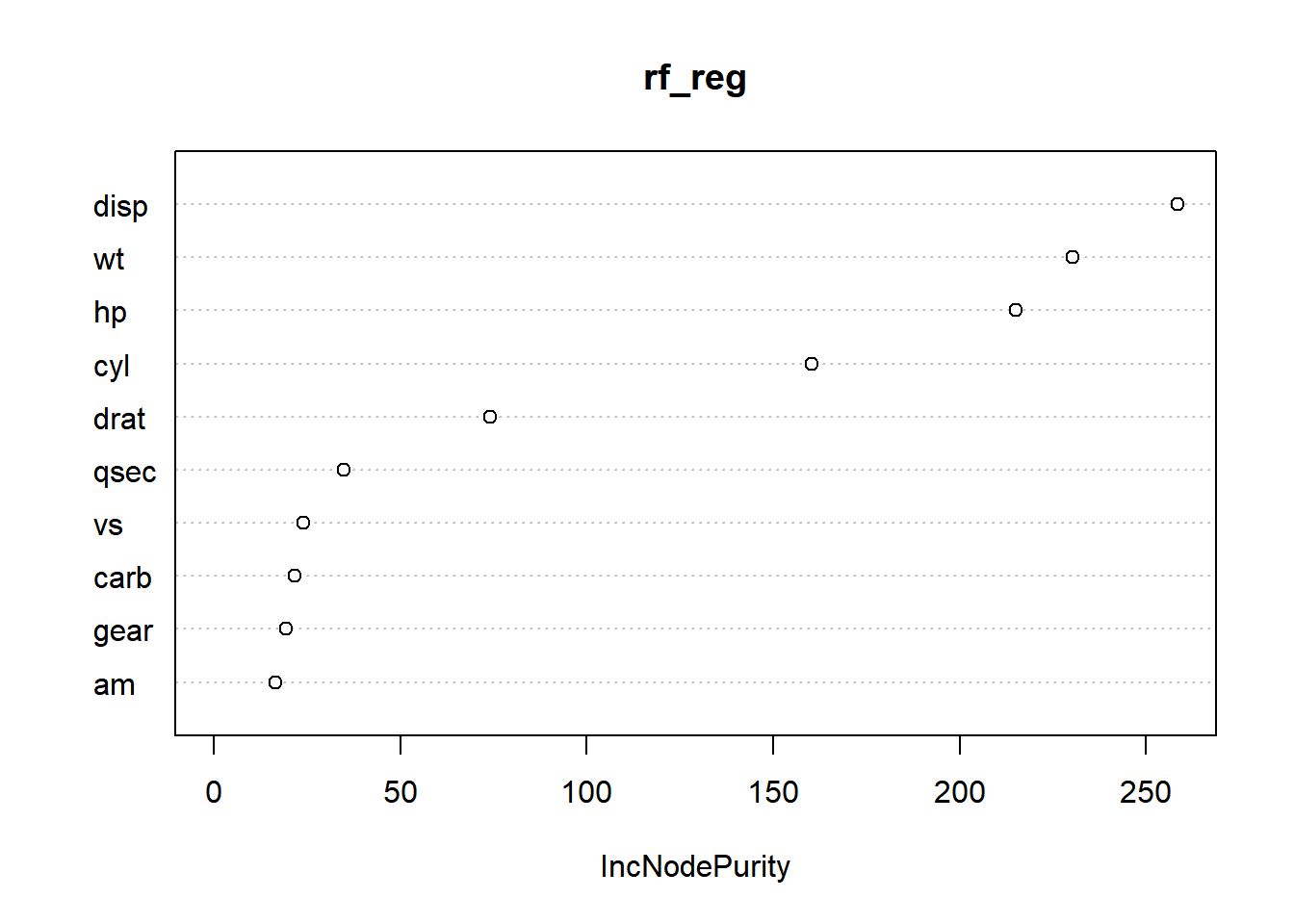
# Feature importancevarImpPlot(rf_reg)
Loading the ‘randomForest’ Library: The line library(randomForest) loads the ‘randomForest’ library into the R environment. This library is necessary to use the Random Forest algorithm.
Loading the ‘mtcars’ Dataset: The command data(mtcars) loads the built-in ‘mtcars’ dataset in R. This dataset contains information about various car models and their attributes, such as miles per gallon (mpg), horsepower (hp), weight (wt), and other specifications.
Fitting Random Forest for Regression (Predicting ‘mpg’): The line rf_reg <- randomForest(mpg ~ ., data = mtcars) fits a Random Forest regression model. It predicts the target variable ‘mpg’ (miles per gallon) based on all available predictor variables denoted by the . in the formula. This implies that all other variables in the ‘mtcars’ dataset, excluding ‘mpg’, are used to predict ‘mpg’ in the regression model.
Setting Seed for Reproducibility: The command set.seed(123) sets the random seed to 123 for reproducibility purposes. Setting the seed ensures that the random number generation used within the Random Forest algorithm follows the same sequence of numbers each time the code is run with the same data and parameters, aiding in reproducibility of results.
Displaying Summary Information of the Model: The line print(rf_reg) displays a summary of the fitted Random Forest regression model (rf_reg). This summary typically includes information about the number of trees in the forest, the importance of variables, mean decrease in accuracy, and other relevant details related to the performance and structure of the Random Forest model.
# Feature importancevarImpPlot(rf_reg)
Feature Importance Calculation:
After fitting the Random Forest regression model (rf_reg) earlier in the code, the function varImpPlot() is used specifically for Random Forest models to visualize the importance of each predictor variable (feature) in influencing the model’s predictions.
Generating the Plot:
The varImpPlot() function generates a graphical representation of variable importance. It plots a bar chart or another suitable visualization where the y-axis typically represents the predictor variables (features), and the x-axis indicates the measure of importance.
Understanding Feature Importance:
The length or height of the bars in the plot corresponds to the importance of each predictor variable. Longer bars signify higher importance, indicating that those variables have a more significant impact on predicting the target variable (‘mpg’ in this case) within the Random Forest regression model.
Interpreting the Plot:
This plot helps in identifying which predictor variables (features) are more influential in predicting the target variable. It provides insights into the relative importance or contribution of each variable in explaining the variability of the target variable based on the Random Forest model’s perspective.
Utilization for Model Interpretation:
Understanding feature importance assists in feature selection, identifying important variables for predictive modeling, and gaining insights into which variables contribute most significantly to the model’s predictive power.
In summary, the varImpPlot(rf_reg) code generates a graphical representation (plot) illustrating the importance of predictor variables within the Random Forest regression model (rf_reg), aiding in understanding the relative impact of each feature on predicting the target variable (‘mpg’) based on the fitted Random Forest model.
Upon examining the plot, it’s noticeable that disp, wt, hp, and cyl emerge as more important features due to their substantial contributions in enhancing node purity within the regression model. These features exhibit a significant increase in node purity after their respective splits, indicating their strong influence in creating more homogeneous subsets within the data, which consequently leads to better predictions of the target variable (mpg in this case).
On the other hand, drat, qsec, vs, carb, gear, and am also play a role in improving node purity within the regression model, albeit to a lesser extent. While these features contribute to purity enhancement through splits, their impact on refining node purity is notably lower compared to the more influential predictors.
In summary, within the regression context, disp, wt, hp, and cyl stand out as the more influential features significantly boosting node purity in the Random Forest model, while drat, qsec, vs, carb, gear, and am contribute to purity improvement to a lesser degree compared to the former set of features.
How does the application of a Random Forest classification model on the iris dataset, with the aim of predicting Species based on various predictor variables, provide insights into the model’s performance, accuracy in classifying species, and the evaluation through a confusion matrix?
# Load the 'iris' datasetdata(iris)# Convert 'Species' to a factor for classificationiris$Species <-as.factor(iris$Species)# Fit Random Forest for classification (predicting species)set.seed(123) # For reproducibilityrf_clf <-randomForest(Species ~ ., data = iris)# Summary of the modelprint(rf_clf)
Call:
 randomForest(formula = Species ~ ., data = iris)
               Type of random forest: classification
                     Number of trees: 500
No. of variables tried at each split: 2

        OOB estimate of  error rate: 4.67%
Confusion matrix:
           setosa versicolor virginica class.error
setosa         50          0         0        0.00
versicolor      0         47         3        0.06
virginica       0          4        46        0.08
# Confusion matrix for evaluationpred <-predict(rf_clf, newdata = iris)#table(iris$Species, pred)
In this example, we use the iris dataset to perform classification on the Species variable using all other available variables. The randomForest() function constructs a classification model, and predict() generates predictions. The table() function creates a confusion matrix to evaluate the model’s performance by comparing actual vs. predicted values.
Load the ‘iris’ dataset: The data(iris) command loads the built-in ‘iris’ dataset in R. This dataset contains measurements of iris flowers, including sepal and petal dimensions, along with the species of the iris (setosa, versicolor, or virginica).
Convert ‘Species’ to a factor for classification: The line iris$Species <- as.factor(iris$Species) converts the ‘Species’ column in the ‘iris’ dataset to a categorical factor. This step is essential for classification tasks, as it prepares the target variable (‘Species’) to be used in a machine learning model.
Fit Random Forest for classification (predicting species): The code randomForest(Species ~ ., data = iris) fits a Random Forest model for classification. It aims to predict the species (‘Species’) of iris flowers based on the other available variables (sepal length, sepal width, petal length, and petal width denoted by the . in the formula) present in the ‘iris’ dataset.
Set seed for reproducibility: The set.seed(123) command ensures that the Random Forest model’s random initialization remains consistent across different runs for reproducibility purposes. This seed allows the random number generation to produce the same sequence of numbers, ensuring the same model output each time it is run with the same data and parameters.
Summary of the model: The print(rf_clf) command displays a summary of the Random Forest model (rf_clf). This summary typically includes information about the number of trees, the number of variables used at each split, and other relevant parameters of the model.
Confusion matrix for evaluation: The code pred <- predict(rf_clf, newdata = iris) generates predictions using the trained Random Forest model (rf_clf) on the same dataset used for training (iris). These predictions are stored in the pred variable. Furthermore, it calculates a confusion matrix, a table used to evaluate the classification model’s performance by comparing predicted class labels against the actual class labels present in the dataset.
It’s worth noting that in practice, for model evaluation, it’s advisable to split the dataset into separate training and testing sets. Using the same dataset for training and evaluation, as demonstrated here, may lead to overly optimistic performance metrics and not accurately represent the model’s performance on unseen data.