The Rayleigh fading channel model is a widely used mathematical model in wireless communication and signal propagation. It describes the variability in the received signal power due to multipath propagation and random fluctuations. The Rayleigh fading model is often employed when there is no dominant line-of-sight component in the wireless channel, and the signal encounters multiple scattered paths with different amplitudes and phases.
B.2 Definition
The Rayleigh fading channel model is a statistical model that characterizes the behavior of a wireless communication channel affected by multipath propagation and random fluctuations. It assumes that the amplitude of the received signal follows a Rayleigh distribution, which is a special case of the more general Ricean distribution. In a Rayleigh fading channel, the received signal power varies randomly over time due to constructive and destructive interference of the multipath components.
In this model, the channel response is characterized by a complex random variable with a Rayleigh distribution. The Rayleigh distribution describes the amplitude of the received signal in a fading channel when there is no dominant line-of-sight component.
B.3 Key Characteristics:
Multipath Propagation: The signal reaches the receiver via multiple paths, each with different distances and phases. This results in constructive or destructive interference at the receiver.
Amplitude Distribution: The amplitudes of the individual multipath components are considered to be independent and identically distributed (i.i.d.) complex Gaussian random variables.
No Line-of-Sight (LoS) Component: The Rayleigh fading model assumes that there is no dominant direct line-of-sight path between the transmitter and the receiver.
Time Variability: The fading process changes over time due to movement of the transmitter, receiver, or objects in the environment.
Mathematically, the probability density function (PDF) of the Rayleigh distribution for the amplitude of the received signal can be expressed as:
\(\sigma\) s the scale parameter of the Rayleigh distribution, related to the average received signal power.
It’s important to note that the Rayleigh fading model provides a simplified representation of real-world wireless channels, and there are variations and extensions of the model to account for more complex scenarios, such as the Ricean fading model (which includes a line-of-sight component) and Nakagami-m fading (a generalized fading model).
The Rayleigh fading model is widely used in the analysis and simulation of wireless communication systems to assess their performance in realistic environments with multipath propagation and fading effects.
B.4 Simple Example one signal.
Let’s consider an example where you have a complex-valued signal with a real part of 3 and an imaginary part of 1. We’ll assume that the signal experiences Rayleigh fading as it passes through the channel. Keep in mind that in a real-world scenario, the fading would be influenced by various factors such as the environment, antenna placement, frequency, and more.
Here’s how you can apply Rayleigh fading to the given signal in R:
# Simulate Rayleigh fading channel effectsimulate_rayleigh_channel <-function(signal_real, signal_imaginary) {# Generate a complex channel response with Rayleigh distribution channel_response <-complex(re =rnorm(1), # Real part with zero mean and unit varianceim =rnorm(1) # Imaginary part with zero mean and unit variance )# Multiply the signal by the channel response received_signal <-complex(re =Re(channel_response) * signal_real -Im(channel_response) * signal_imaginary,im =Re(channel_response) * signal_imaginary +Im(channel_response) * signal_real )return(received_signal)}# Given datasignal_real <-3signal_imaginary <-1# Simulate Rayleigh fadingreceived_signal <-simulate_rayleigh_channel(signal_real, signal_imaginary)# Print the received signalcat("Received Signal (Real Part):", Re(received_signal), "\n")
Received Signal (Real Part): 2.160657
cat("Received Signal (Imaginary Part):", Im(received_signal), "\n")
Received Signal (Imaginary Part): -0.7754732
In this example, the simulate_rayleigh_channel function generates a complex channel response with Rayleigh distribution characteristics and applies it to the given signal. The resulting received signal will have both real and imaginary parts affected by the channel fading.
This complex number captures the magnitude and phase changes introduced by the wireless channel. The real and imaginary parts correspond to the amplitude and phase of the channel response, respectively.
When you multiply the original transmitted signal (which is also a complex number) by the complex channel response, you effectively combine the amplitude and phase effects of the channel with the original signal. This multiplication accounts for both amplitude scaling (signal strength changes) and phase shifts (signal propagation delays and phase rotations).
Keep in mind that each time you run this simulation, you’ll get different results due to the randomness of the Rayleigh distribution. This simulation provides a basic illustration of how the Rayleigh fading channel affects a complex-valued signal. In practice, more complex models and simulations should be used to accurately capture the behavior of a wireless communication channel.
Now we are ready to pass a bunch of data.
B.5 Modeling digital communication systems
On this section we will simulate passing a bunch of digital data by using Quadrature Amplitude Modulation (QAM).
QAM is a digital modulation scheme used in telecommunications and signal processing. It conveys data by varying the amplitude of two carrier waves (in-phase and quadrature) simultaneously, allowing multiple bits to be encoded in a single symbol, making it an efficient way to transmit digital information over communication channels.
library(MASS)library(ggplot2)# INPUT of 16 SIGNALSmean_set_QAM <-c(-3-3i, -3-1i, -3+1i, -3+3i, -1-3i, -1-1i, -1+1i, -1+3i,1-3i, 1-1i, 1+1i, 1+3i, 3-3i, 3-1i, 3+1i, 3+3i)# Definition of data generatorgenerate_real_samples_with_labels_Rayleigh <-function(number) { h_r <-rnorm(number, sd =sqrt(2)/20) # Rayleigh spread for the real h_i <-rnorm(number, sd =sqrt(2)/20) # Rayleigh spread for the imag h_complex <- h_r +1i * h_i labels_index <-sample(seq_along(mean_set_QAM), number, replace =TRUE) data <- mean_set_QAM[labels_index] received_data <- h_complex * data # Total Effect! received_data <-cbind(Re(received_data), Im(received_data)) gaussian_random_noise <-mvrnorm(number, mu =c(0, 0), Sigma =matrix(c(0.01, 0, 0, 0.01), ncol =2)) #MASS received_data <- received_data + gaussian_random_noise conditioning <-cbind(Re(data), Im(data), h_r, h_i) #by binding I can effectively label each data-rowreturn(list(received_data, conditioning))}
Let’s break down each part of the code:
mean_set_QAM: This is an array of complex numbers representing the constellation points for a 16-QAM (Quadrature Amplitude Modulation) scheme. Each complex number represents a possible symbol that can be transmitted.
h_r and h_i: These are arrays of real numbers generated from a normal distribution with a standard deviation of sqrt(2)/20. They spread the original signal. These arrays represent the real and imaginary components of the complex channel coefficients.
h_complex: This creates an array of complex numbers by combining the h_r (real) and h_i (imaginary) components, resulting in a complex channel coefficient for each element.
labels_index: This line generates an array of random integers, each representing an index from the mean_set_QAM array. This indicates which symbol will be transmitted for each channel use. It’s as if you’re selecting random symbols from the QAM constellation for transmission.
data: This line extracts the symbols from mean_set_QAM based on the indices provided by labels_index. In other words, it creates the data that is going to be transmitted through the channel.
received_data: This line simulates the received data after passing through the channel. It multiplies the complex channel coefficients (h_complex) with the transmitted QAM symbols (data). This simulates the total effect of the channel on the transmitted symbols, including noise and potential distortion.
In summary, this code simulates a communication system where QAM symbols are transmitted through a complex channel characterized by random channel coefficients. The received data is then calculated by applying these channel coefficients to the transmitted symbols. This type of simulation is commonly used to analyze the performance of communication systems in the presence of noise and channel impairments.
B.6 Constelation plot
samples <-14000tuple <-generate_real_samples_with_labels_Rayleigh(samples)spread_real <- tuple[[2]][,1]+tuple[[2]][,3]spread_imag <- tuple[[2]][,2]+tuple[[2]][,4]df_const <-data.frame(real=spread_real,imag=spread_imag)plot(df_const,cex=0.2, asp =1, xlim=c(-4, 4),ylim=c(-4,4), main="Channel Response: Spread due Rayleigh Distribution")
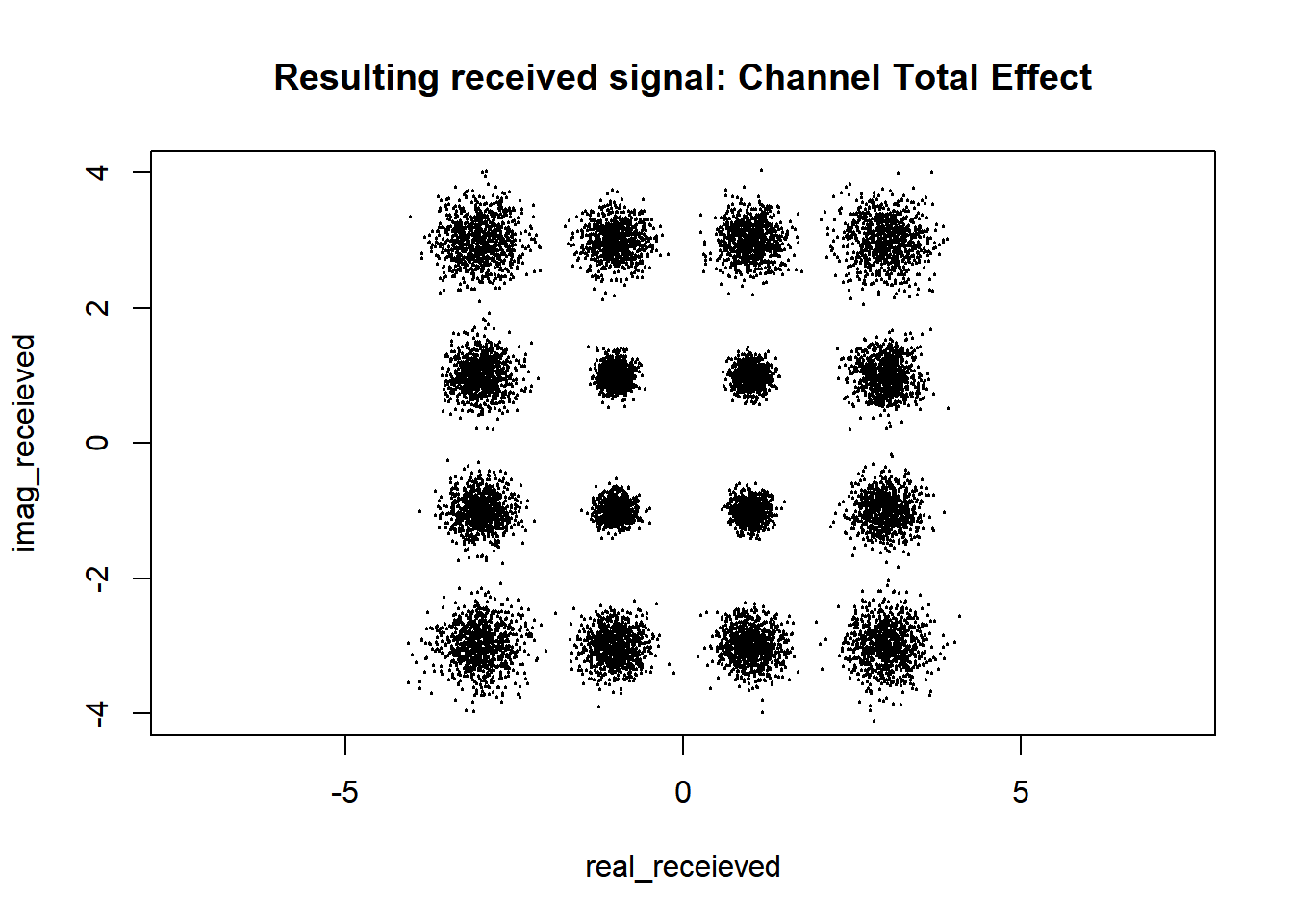
df_received <-data.frame(real_receieved = tuple[[1]][,1]+tuple[[2]][,1], imag_receieved = tuple[[1]][,2]+tuple[[2]][,2])plot(df_received,cex=0.2, asp =1, xlim=c(-4, 4),ylim=c(-4,4), main="Resulting received signal: Channel Total Effect")