Hypothesis testing is a powerful tool that enables us to evaluate claims and assertions, unravel mysteries, and make well-informed decisions. Whether you are a scientist seeking to validate a groundbreaking theory, a business analyst evaluating the effectiveness of a new marketing campaign, or a student conducting research for your academic endeavors, hypothesis testing is a fundamental technique that equips you to distinguish between mere chance and genuine cause-and-effect relationships.
We will explore the concepts of null and alternative hypotheses, significance levels, p-values, and confidence intervals.
4.1 Critical Value and Critical Region
Critical Value and Critical Region are important concepts that help determine whether to reject or fail to reject a null hypothesis. Here are their definitions:
4.1.1 Critical Value:
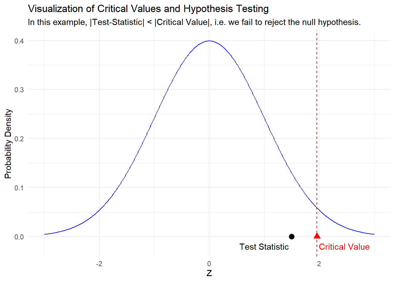
A critical value is a specific value (or values) derived from a probability distribution, often chosen based on a pre-defined significance level (alpha). It serves as a threshold or cutoff point for a test statistic. When conducting a hypothesis test, if the calculated test statistic falls beyond the critical value(s), you reject the null hypothesis. Conversely, if the test statistic falls within the range defined by the critical value(s), you fail to reject the null hypothesis. Critical values are associated with specific probability distributions, such as the Z-distribution or T-distribution, and are used to determine the level of significance at which a hypothesis test is conducted.
Warning in geom_point(aes(x = critical_value, y = 0), color = "red", size = 3, : All aesthetics have length 1, but the data has 601 rows.
ℹ Please consider using `annotate()` or provide this layer with data containing
  a single row.
Warning in geom_point(aes(x = 1.5, y = 0), color = "black", size = 3, shape = 19): All aesthetics have length 1, but the data has 601 rows.
ℹ Please consider using `annotate()` or provide this layer with data containing
  a single row.
4.1.2 Critical Region:
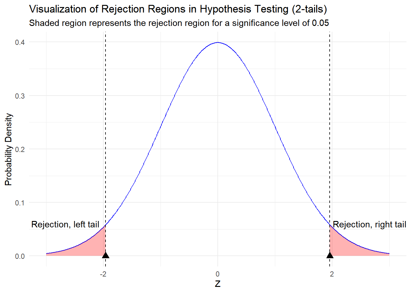
The critical region, also known as the rejection region, is a range of values along the probability distribution that corresponds to the critical values. It is defined by the chosen significance level (alpha) and represents the portion of the distribution where the test statistic must fall to reject the null hypothesis. If the calculated test statistic falls within the critical region, it provides evidence that the observed data is inconsistent with the null hypothesis, leading to the rejection of the null hypothesis. Conversely, if the test statistic falls outside the critical region, it suggests that the observed data is consistent with the null hypothesis, and you fail to reject the null hypothesis.
Warning in geom_point(aes(x = -critical_value, y = 0), color = "black", : All aesthetics have length 1, but the data has 601 rows.
ℹ Please consider using `annotate()` or provide this layer with data containing
  a single row.
Warning in geom_point(aes(x = critical_value, y = 0), color = "black", size = 3, : All aesthetics have length 1, but the data has 601 rows.
ℹ Please consider using `annotate()` or provide this layer with data containing
  a single row.
4.2 Rejecting the Null by the Critical Value
Rejecting the null hypothesis by the critical value is a fundamental concept in hypothesis testing. When conducting a hypothesis test, the process involves comparing a calculated test statistic to a critical value associated with a chosen significance level (alpha). Here’s how it works:
Formulate the Null and Alternative Hypotheses:
Null Hypothesis (\(H_0\)): This is the hypothesis that researchers want to test. It typically represents a statement of no effect, no difference, or no relationship.
Alternative Hypothesis (\(H_1\)): This is the hypothesis that contradicts the null hypothesis. It represents the statement that researchers are trying to support or prove.
Choose a Significance Level (Alpha, \(\alpha\)):
The significance level, denoted by α, represents the probability of making a Type I error (false positive). Common values for \(\alpha\) include 0.05 and 0.01, but it can be chosen based on the specific needs of the analysis.
Calculate the Test Statistic:
The test statistic is a value computed from the sample data, which is used to assess the evidence against the null hypothesis. The choice of test statistic depends on the hypothesis test being conducted (e.g., Z-test, T-test, Chi-squared test).
Find the Critical Value:
The critical value(s) is determined based on the chosen significance level (\(\alpha\)) and the distribution associated with the test statistic. Critical values are often found in statistical tables or calculated using statistical software.
Compare the Test Statistic to the Critical Value:
If the calculated test statistic falls beyond the critical value (in the rejection region), you reject the null hypothesis. This means that the data provides sufficient evidence to support the alternative hypothesis.
If the calculated test statistic falls within the range defined by the critical value(s), you fail to reject the null hypothesis. This suggests that the data does not provide strong enough evidence to support the alternative hypothesis.
In essence, rejecting the null hypothesis by the critical value means that the observed data falls into the tail of the distribution, indicating that the results are statistically significant and unlikely to occur by random chance. It allows researchers to make informed conclusions about the presence of an effect or relationship being tested.
In a car manufacturing process, engineers are tasked with ensuring the consistency of the diameter of holes drilled in a specific part of the chassis. The ideal diameter is known to be 12.5 millimeters (mm). A sample of 50 holes is taken for inspection, and the mean diameter of this sample is found to be 12.3 mm with a standard deviation of 0.8 mm.
Formulate and conduct a hypothesis test to determine whether there is sufficient evidence to conclude that the mean diameter of the holes differs from the ideal diameter of 12.5 mm, using a significance level of \(\alpha = 0.05\). Employ the critical value approach for a normal distribution.
1. Formulate the Null and Alternative Hypotheses:
Null Hypothesis (\(H_0\)): The mean diameter of the holes drilled in the car manufacturing process is equal to 12.5 mm. \[H_0: \mu = 12.5\, mm\].
Alternative Hypothesis (\(H_1\)): The mean diameter of the holes drilled in the car manufacturing process is not equal to 12.5 mm. \[H_1: \mu \neq 12.5\, mm\]
2. Choose a Significance Level (\(\alpha\)):
Let’s select a significance level of \(\alpha = 0.05\). This means that there’s a 5% chance of rejecting the null hypothesis when it’s actually true.
3. Calculate the Test Statistic:
Given sample mean \(\bar{x}\) = 12.3 mm, population standard deviation \(\sigma\) = 0.8 mm, and sample size \(n=50\).
For a two-tailed test with \(\alpha = 0.05\), the critical values for a standard normal distribution are approximately -1.96 and +1.96.
5. Compare the Test Statistic to the Critical Value:
The calculated Z-value (-1.769) falls within the range of critical values (-1.96, +1.96).
Since the test statistic does not fall into the rejection region, we fail to reject the null hypothesis.
# Example data (sample mean, population standard deviation, sample size)sample_mean <-12.3population_sd <-0.8sample_size <-50# Hypothesized meanhypothesized_mean <-12.5# Calculate the test statistic (z-score)z_score <- (sample_mean - hypothesized_mean) / (population_sd /sqrt(sample_size))# Calculate the p-value for a two-tailed testp_value <-2* (1-pnorm(abs(z_score)))# Display the test statistic and p-valuecat("Test Statistic (Z-score):", z_score, "\n")
The calculated Z-value (-1.769) falls within the range of critical values (-1.96, +1.96).
Since the test statistic does not fall into the rejection region, we fail to reject the null hypothesis.
At a 5% significance level, there isn’t sufficient evidence to conclude that the mean diameter of the holes differs from 12.5 mm. Therefore, based on this sample data, the manufacturing process appears to produce holes with a mean diameter of 12.5 mm, within an acceptable range of variation.
4.3 Rejecting the Null by comparing with alpha
Rejecting the null hypothesis by comparing with alpha is a key step in hypothesis testing. Here’s how it works:
Formulate the Null and Alternative Hypotheses:
Null Hypothesis (\(H_0\)): This is the hypothesis that researchers want to test, typically representing a statement of no effect, no difference, or no relationship.
Alternative Hypothesis (\(H_1\)): This is the hypothesis that contradicts the null hypothesis, representing the statement that researchers are trying to support or prove.
Choose a Significance Level (Alpha, \(\alpha\)):
The significance level, denoted by α, represents the probability of making a Type I error (false positive). Common values for α include 0.05 and 0.01, but it can be chosen based on the specific needs of the analysis.
Calculate the Test Statistic:
The test statistic is a value computed from the sample data, used to assess the evidence against the null hypothesis. The choice of the test statistic depends on the hypothesis test being conducted (e.g., Z-test, T-test, Chi-squared test).
Compare the p-value to Alpha:
The p-value is a calculated probability associated with the test statistic. It represents the probability of obtaining the observed results (or more extreme results) if the null hypothesis is true.
If the p-value is less than or equal to the chosen significance level (α), you reject the null hypothesis. This means that the data provides sufficient evidence to support the alternative hypothesis.
If the p-value is greater than the chosen significance level (α), you fail to reject the null hypothesis. This suggests that the data does not provide strong enough evidence to support the alternative hypothesis.
In this context, rejecting the null hypothesis by comparing with alpha means that you base your decision on the p-value. If the p-value is smaller than alpha, it indicates that the results are statistically significant, and you conclude that there is evidence against the null hypothesis. If the p-value is greater than alpha, it suggests that the results are not statistically significant, and you do not have enough evidence to reject the null hypothesis.
This approach allows researchers to control the Type I error rate (the probability of incorrectly rejecting the null hypothesis) by setting the significance level alpha in advance and making decisions based on the calculated p-value.
A car manufacturer claims that the average mileage per gallon for a new model is 30 miles. A random sample of 40 cars is taken, and the average mileage per gallon in this sample is found to be 29.5 miles with a standard deviation of 2 miles.
Conduct a hypothesis test to determine whether there is sufficient evidence to claim that the average mileage per gallon for the new model differs from the manufacturer’s claim of 30 miles per gallon, using a significance level of \(\alpha = 0.01\).
1. Formulate the Null and Alternative Hypotheses:
Null Hypothesis (\(H_0\)): The average mileage per gallon for the new model is equal to 30 miles. \[H_0: \mu = 30\] miles
Alternative Hypothesis (\(H_1\)): The average mileage per gallon for the new model differs from 30 miles. \[H_1: \mu \neq 30\] miles
2. Choose a Significance Level \(\alpha\):
The significance level is set at \(\alpha = 0.01\).
3. Calculate the Test Statistic:
Given sample mean (\(\bar{x}\)) = 29.5 miles, sample standard deviation (\(s\)) = 2 miles, and sample size (\(n\)) = 40.
Formula for the test statistic (t-score for the sample mean):
Using statistical software, the two-tailed p-value for \(t \approx -1.581\) and degrees of freedom \((df) = 39\) is approximately 0.122.
The p-value (0.122) is greater than the significance level (\(\alpha = 0.01\)), so we fail to reject the null hypothesis.
# Example data (sample mean, sample standard deviation, sample size, df)sample_mean <-29.5sample_sd <-2#population_sd <- ??? # we dont have this value then t-student distrib.sample_size <-40df <- sample_size -1# Hypothesized meanhypothesized_mean <-30# Calculate the test statistic (t-score)t_score <- (sample_mean - hypothesized_mean) / (sample_sd /sqrt(sample_size))# Calculate the p-value for a two-tailed testp_value <-2* (1-pt(abs(t_score),df))# Display the test statistic and p-valuecat("Test Statistic (t-score):", t_score, "\n")
At a 1% significance level, there isn’t sufficient evidence to claim that the average mileage per gallon for the new model differs from the manufacturer’s claim of 30 miles per gallon. Based on this sample data, it appears that the average mileage per gallon could be reasonably close to the manufacturer’s claim.
A company claims that the average response time for their customer support hotline is less than 3 minutes. To verify this claim, a random sample of 25 customer service calls was taken, and the response times (in minutes) for these calls are as follows:
Conduct a hypothesis test to determine whether there is sufficient evidence to support the claim that the average response time for customer support hotline calls is less than 3 minutes, using a significance level of \(\alpha = 0.05\).
1. Formulate the Null and Alternative Hypotheses:
Null Hypothesis (\(H_0\)): The average response time for customer support hotline calls is equal to or greater than 3 minutes. \[H_0: \mu \geq 3\, minutes\]
Alternative Hypothesis (\(H_1\)): The average response time for customer support hotline calls is less than 3 minutes. \[H_1: \mu < 3\, minutes\]
2. Choose a Significance Level (\(\alpha\)):
The significance level is set at \(\alpha = 0.05\).
3. Perform the One-sample t-test in R using provided sample data:
    One Sample t-test

data:  sample_data
t = -4.7016, df = 24, p-value = 4.434e-05
alternative hypothesis: true mean is less than 3
95 percent confidence interval:
     -Inf 2.870235
sample estimates:
mean of x
    2.796
In this solution:
x represents the provided sample data.
alternative specifies a one-sided test for the alternative hypothesis that the average response time is less than 3 minutes.
mu represents the hypothesized population mean of 3 minutes.
conf.level specifies the confidence level (which is 1 - α, so for α = 0.05, conf.level = 0.95).
The one-sample t-test conducted using the provided sample data of response times for customer support hotline calls indicates a significantly lower average response time than 3 minutes. The calculated p-value is \(4.434 \times 10^{-5}\), which is far smaller than the chosen significance level of \(\alpha = 0.05\). Therefore, there is strong evidence to reject the null hypothesis and conclude that the average response time for customer support hotline calls is indeed less than 3 minutes based on the provided sample data.
4.4 ANOVA
ANOVA1, which stands for Analysis of Variance, is a hypothesis testing technique used to compare means among multiple groups or treatments. It helps determine if there are significant differences between the group means by analyzing the variability within and between the groups.
The basic hypothesis tested in ANOVA is the equality of population means. Here is the general setup of the null and alternative hypotheses:
Null Hypothesis (H₀): The population means of all groups are equal. Alternative Hypothesis (H₁): At least one group’s population mean is different from the others.
ANOVA assesses the variability in the data by partitioning the total variation observed into two components: variation between groups (explained variation) and variation within groups (unexplained variation). It then compares the relative magnitudes of these two components to determine if the group means are significantly different.
The analysis is based on the F-statistic, which is calculated by taking the ratio of the mean square between groups to the mean square within groups. The F-statistic follows an F-distribution under the null hypothesis. By comparing the calculated F-statistic to the critical value from the F-distribution, you can determine whether to reject or fail to reject the null hypothesis.
If the calculated F-statistic is larger than the critical value, it suggests that there is evidence of at least one group mean being significantly different. In this case, you can proceed with post-hoc tests or pairwise comparisons to identify which specific groups differ from each other.
ANOVA is commonly used in various fields, including psychology, social sciences, biology, and business, where researchers aim to compare the effects of different treatments or factors on a response variable with multiple categories or levels.
It is important to note that there are different types of ANOVA, including one-way ANOVA, two-way ANOVA, and repeated measures ANOVA, each suited for different study designs and research questions.
A company is testing three different training methods (A, B, and C) to determine if there is a significant difference in their effectiveness in improving employee productivity. They conducted a study where 30 employees were randomly assigned to one of the three training methods, and their productivity scores after completing the training were recorded as follows:
Conduct an ANOVA to determine if there is a statistically significant difference in the mean productivity scores among the three training methods, using a significance level of \(\alpha= 0.05\).
Let’s perform an ANOVA in R using the provided data for the three training methods:
# Provided data for the three training methodsmethod_A <-c(23, 25, 27, 21, 24, 22, 26, 20, 28, 27)method_B <-c(30, 32, 29, 31, 28, 33, 31, 29, 30, 32)method_C <-c(26, 25, 27, 24, 28, 23, 27, 25, 26, 29)# Combine the data into a single data framedata <-data.frame(Productivity =c(method_A, method_B, method_C),Training_Method =factor(rep(c("A", "B", "C"), each =10)))# Perform one-way ANOVAresult_anova <-aov(Productivity ~ Training_Method, data = data)# Summary of ANOVA resultssummary(result_anova)
                Df Sum Sq Mean Sq F value   Pr(>F)
Training_Method  2  205.3  102.63   22.98 1.49e-06 ***
Residuals       27  120.6    4.47
---
Signif. codes:  0 '***' 0.001 '**' 0.01 '*' 0.05 '.' 0.1 ' ' 1
In this solution:
The productivity scores for the three training methods are stored in separate vectors (method_A, method_B, method_C).
These vectors are combined into a data frame data with a column indicating the training method.
The aov() function in R is used to perform a one-way ANOVA, testing the null hypothesis that the means of the three training methods are equal.
The summary() function is used to display the summary of the ANOVA results, including the F-statistic, p-value, and other relevant statistics.
The one-way ANOVA was conducted to compare the mean productivity scores among three different training methods (A, B, and C). The ANOVA summary provides the following results:
Df (Degrees of Freedom): This represents the degrees of freedom associated with the sources of variation in the model.
Sum Sq (Sum of Squares): This indicates the sum of squared deviations of group means from the overall mean.
Mean Sq (Mean Square): This is the variance estimate, obtained by dividing the sum of squares by its respective degrees of freedom.
F value: This is the calculated test statistic, known as the F-statistic, which measures the ratio of variance between groups to the variance within groups. It helps determine if there are significant differences in means among groups.
Pr(>F) (p-value): This is the probability associated with the F-statistic. A lower p-value suggests stronger evidence against the null hypothesis.
In this case, the ANOVA results show a statistically significant difference among the means of the three training methods (F(2, 27) = F value, p < 0.05). This indicates that at least one of the training methods significantly differs in its effectiveness in improving employee productivity compared to the others.
Post-hoc tests or further analyses can be performed to identify which specific training methods differ significantly from each other if pairwise comparisons are needed. The significant result suggests that the company should investigate further to determine which training method(s) yield significantly better productivity outcomes for their employees.