In the realm of statistical modeling and machine learning, the choice of a loss function plays a pivotal role in shaping the behavior and performance of a model. A loss function quantifies the discrepancy between the predicted values of a model and the actual observed outcomes. From a statistical perspective, loss functions serve as a bridge between the mathematical representation of a model and its alignment with the underlying data distribution.
D.2 Definition of Loss Function
At its core, a loss function measures the dissimilarity between the predicted values (f(x)) produced by a statistical model and the true observed values (y) present in the dataset. In other words, it quantifies the “loss” or “cost” associated with the model’s predictions. Mathematically, the loss function L can be defined as:
\[ L(y, f(x)) \]
where:
y represents the true observed value (ground truth).
f(x) denotes the model’s prediction based on the input x.
The primary objective in statistical modeling is to minimize this loss function, which effectively means reducing the discrepancy between predictions and actual outcomes.
D.3 Importance of Loss Functions
Loss functions serve a dual purpose in statistical modeling:
Objective Function: From an optimization standpoint, the loss function serves as the objective function that the model seeks to minimize. By finding the optimal parameter values that minimize the loss, the model becomes better aligned with the underlying data distribution.
Model Selection and Evaluation: Loss functions enable model selection by providing a quantitative measure of how well a model fits the data. Different loss functions emphasize different aspects of prediction errors (e.g., mean squared error for regression, cross-entropy for classification), allowing practitioners to tailor their models to the specific task at hand.
D.4 Role of Loss Functions in Parameter Estimation
When estimating the parameters of a statistical model, loss functions are used to guide the optimization process. Common optimization techniques such as gradient descent seek to find parameter values that minimize the loss. By minimizing the loss, the model effectively “learns” from the data and captures the underlying relationships between variables.
D.5 Types of Loss Functions
The choice of a loss function depends on the nature of the problem and the type of data. Different loss functions capture different aspects of prediction errors, such as absolute deviations, squared deviations, or likelihood-based measures. Common loss functions include:
Mean Squared Error (MSE): Emphasizes squared deviations between predictions and actual values, commonly used in regression problems.
Mean Absolute Error (MAE): Measures the absolute differences between predictions and actual values, providing a more robust measure against outliers.
Cross-Entropy: Used in classification tasks to measure the dissimilarity between predicted class probabilities and actual class labels.
Log-Likelihood: Often used in maximum likelihood estimation to quantify the likelihood of observed data given the model.
D.6 Example using R
The following example demonstrates the use of the Mean Squared Error (MSE) loss function and how optimization aims to minimize the errors using gradient descent.
We will create a simple linear regression model and use the MSE loss to train the model using gradient descent to fit a line to a set of data points.1
# Generate some example dataset.seed(123)x <-seq(1, 10, by =0.5)y <-2* x +3+rnorm(length(x), mean =0, sd =1)# Define the MSE loss functionmse_loss <-function(y_true, y_pred) {mean((y_true - y_pred)^2)}# Define the model parameters (slope and intercept)slope <-0intercept <-0# Hyperparameterslearning_rate <-0.01num_epochs <-100# Training loopfor (epoch in1:num_epochs) {# Forward pass: compute predictions y_pred <- slope * x + intercept# Compute the MSE loss loss <-mse_loss(y, y_pred)# Compute gradients with respect to parameters d_slope <--2*mean(x * (y - y_pred)) d_intercept <--2*mean(y - y_pred)# Update parameters using gradient descent slope <- slope - learning_rate * d_slope intercept <- intercept - learning_rate * d_intercept# Print progresscat(sprintf("Epoch %d - Loss: %.4f\n", epoch, loss))}
# Final trained model parameterscat("Trained Slope:", slope, "\n")
Trained Slope: 2.272553
cat("Trained Intercept:", intercept, "\n")
Trained Intercept: 1.291805
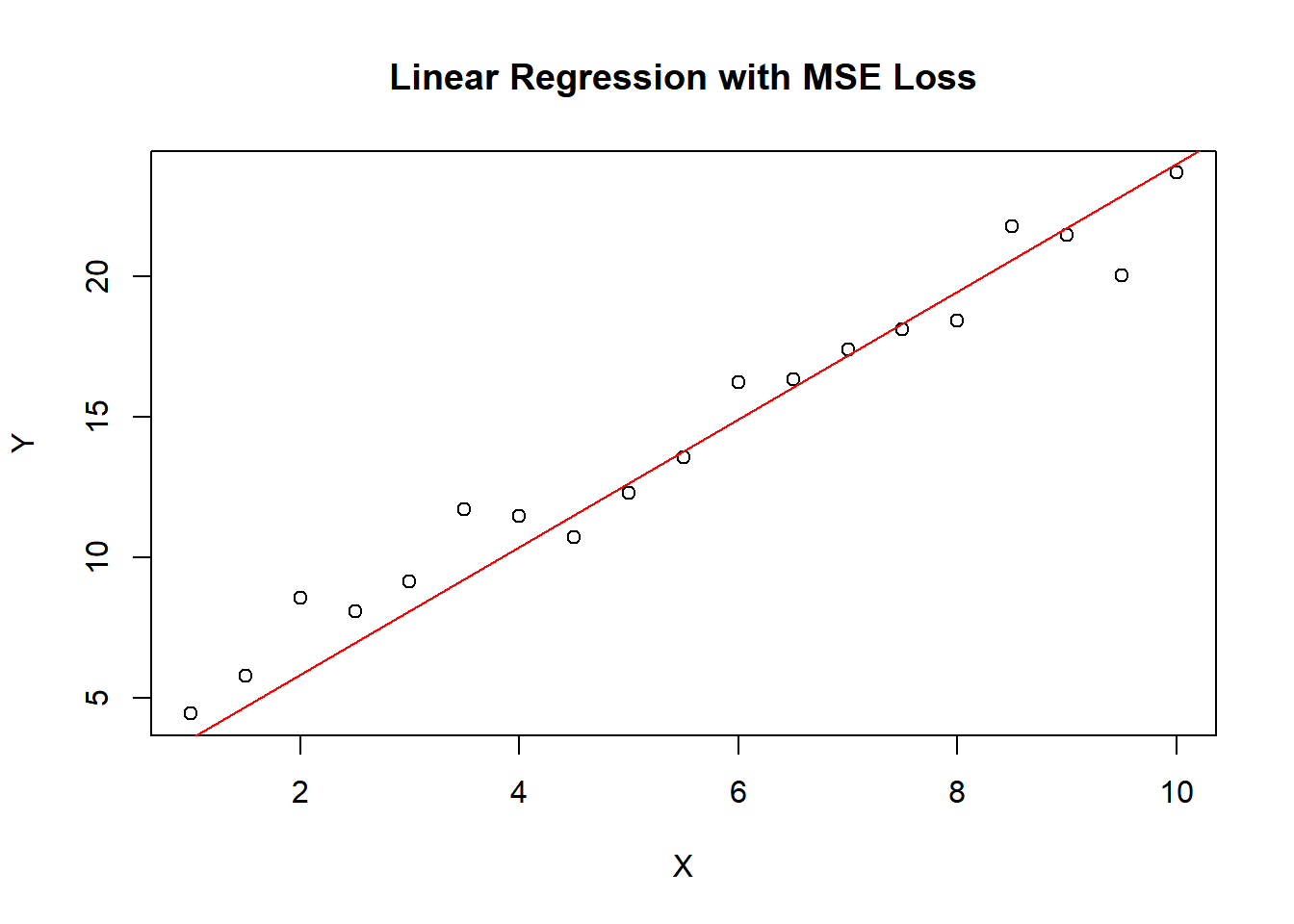
# Plot the original data and the fitted lineplot(x, y, main ="Linear Regression with MSE Loss", xlab ="X", ylab ="Y")abline(a = intercept, b = slope, col ="red")
df <-data.frame(x,y)library(plotly)library(dplyr)fig <-plot_ly(data = df, x =~x, y =~y, type ='scatter', alpha =0.65, mode ='markers', name='data')fig <- fig %>%add_trace(data = df, x =~x, y =~x*slope+intercept, name ='Lin. Regr. with MSE Loss', color ="red", mode ='lines', alpha =1)fig
In this example, we start with some synthetic data points \((x, y)\) that follow a linear relationship with added noise. We define the MSE loss function and the model parameters (slope and intercept). The training loop iterates for a fixed number of epochs, where we perform a forward pass to compute predictions, calculate the MSE loss, compute gradients, and update the model parameters using gradient descent. The slope and intercept are adjusted iteratively to minimize the MSE loss.
After training, you’ll see that the trained slope and intercept values approximate the original slope and intercept of the linear relationship. The fitted line should align with the data points, indicating successful minimization of the MSE loss through optimization.
D.7 Conclusion
Loss functions are the cornerstone of statistical modeling and machine learning, shaping the behavior of models and guiding their learning process. Their role extends beyond optimization, as they offer insights into the alignment between models and data distributions. A well-chosen loss function not only aids in achieving accurate predictions but also provides a deeper understanding of the underlying statistical relationships.
References and footnotes
We could use the lm() function in R to perform this analysis, but we will not delve into the details of how it is done here.↩︎