3 Normal Distribution

"It is not knowledge, but the act of learning, 
not possession, but the act of getting there, 
which grants the greatest enjoyment."
– Carl Friedrich Gauss

The normal distribution, often referred to as the bell curve or Gaussian distribution, is a fundamental concept in statistics and probability theory. Its symmetric, bell-shaped curve is a hallmark of natural phenomena and random processes. Normal variables, which follow this distribution, can be found throughout various fields of science and engineering. From the distribution of heights in a population to the behavior of particles in physics, from the quality control of manufactured products to the analysis of financial data in economics, the ubiquity of the normal distribution reflects its relevance as a model for understanding and characterizing a wide array of real-world phenomena.

The following chapter aims to provide examples in R on how to solve statistical problems involving random continuous variables that follow a normal distribution. This chapter will be divided into seven sections:

Historical background on normal distributions.
The mathematics of a normal distribution of parameters \(\mu\) and \(\sigma\).
Functions in R which calculate probabilities and properties of normal distributions.
Basic Problems: This section will focus on testing concepts and getting familiar with R functions and definitions.
Normal Problems: Here, we will present a curated selection of typical problems that commonly arise in elementary statistics.
Statistical Significant Problems: In this advanced section, we will cover a set of challenging problems specifically designed for students aiming to excel and be among the top 5% of their class.
List of Machine Learning Algorithms which require that the input data is normal distributed, or they perform better when the data conforms to a normal distribution.

The following minimal definitions and selected problems has been obtain from stats.libretexts.org under Creative Commons 4.0 and ChatGPT.

3.1 Introduction to the `Gaussian` distribution

The concept of the normal distribution, also known as the Gaussian distribution, was pioneered by Carl Friedrich Gauss, in the early 19th century. Gauss’s work on the distribution of errors in astronomical observations led him to develop the foundation of what we now know as the normal distribution.

Gauss’s work on the normal distribution was primarily conducted around the year 1809 in Göttingen, Germany. His insights were later published in his work titled “Theoria Motus Corporum Coelestium in Sectionibus Conicis Solem Ambientium”¹ (Theory of the Motion of Celestial Bodies in Conic Sections Surrounding the Sun), published in 1809.

Gauss’s work laid the groundwork for understanding the distribution of errors and variability in natural phenomena. The normal distribution, often referred to as the bell curve due to its characteristic shape, has since become a fundamental concept in statistics, probability theory, and various scientific disciplines.

The normal distribution’s key features, such as its symmetry and the fact that many natural phenomena exhibit distributions close to the normal, have led to its widespread use. Here are a few of the future applications that stemmed from Gauss’s work:

Statistics and Probability: The normal distribution serves as a foundational distribution in statistics and probability theory. It’s used to model various real-world phenomena, such as measurement errors and random variables.

Central Limit Theorem: Gauss’s work contributed to the development of the Central Limit Theorem, which states that the distribution of the sum (or average) of a large number of independent, identically distributed random variables approaches a normal distribution, regardless of the original distribution.

Data Analysis: The normal distribution is commonly used in data analysis, hypothesis testing, and confidence interval estimation. Many statistical methods and tests assume or approximate a normal distribution.

Quality Control and Manufacturing: The normal distribution is applied in quality control to assess variability and defects in manufacturing processes. It helps in setting acceptable ranges and identifying deviations from the norm.

Social Sciences: Gaussian models are often used to describe and analyze social and psychological phenomena, like intelligence scores, heights, and many other human characteristics.

Financial Markets: In finance, the normal distribution is used in models like the Black-Scholes option pricing model and in risk assessment.

In summary, Gauss’s groundbreaking work on normal distributions in the early 19th century has had a profound impact on a wide range of scientific and practical applications, shaping the way we understand and analyze variability and randomness in various fields.

3.2 The Mathematics

Definition:²

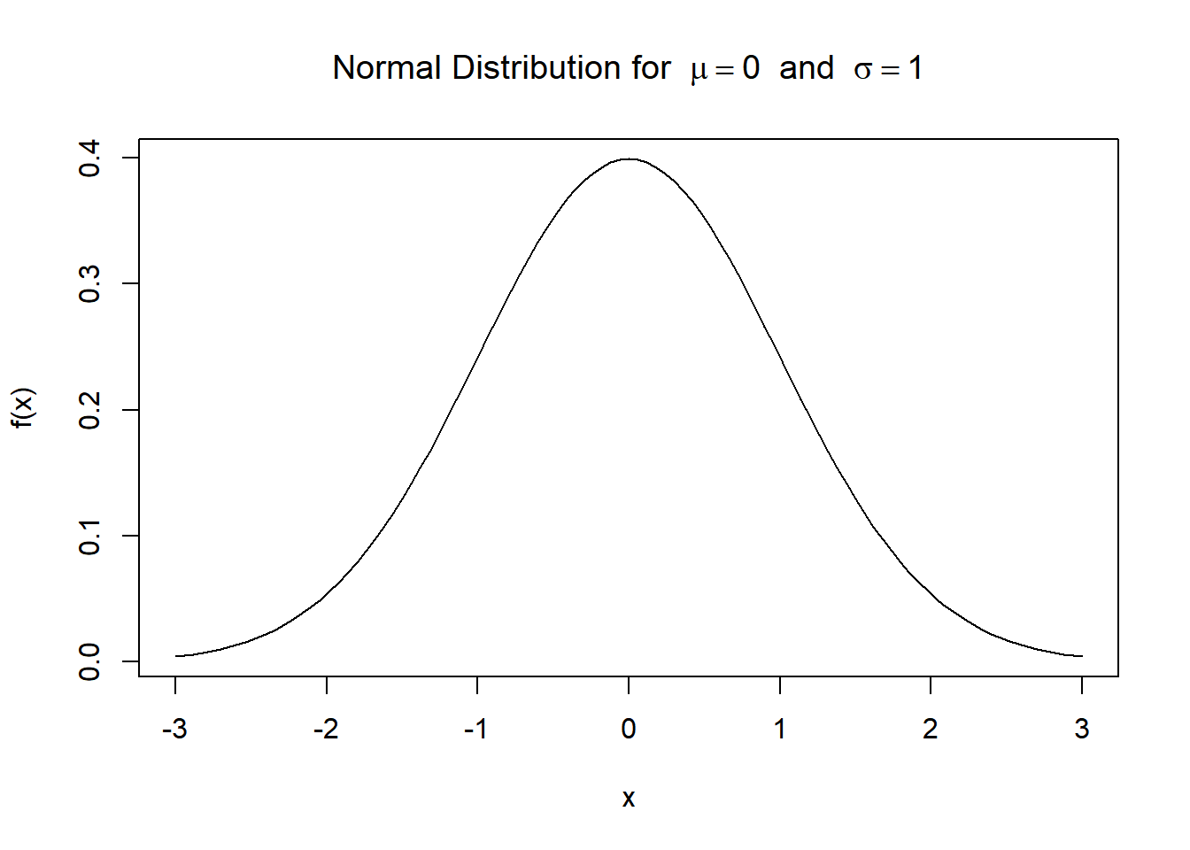
A normally distributed variable, also known as a Gaussian distributed variable or a normally distributed random variable, refers to a continuous probability distribution that is symmetric and bell-shaped. It is characterized by its probability density function, which is described by the bell-shaped curve known as the normal curve or the Gaussian curve.

The definition of a normally distributed variable can be expressed in terms of its probability density function (PDF), denoted as \(f(x)\). For a variable \(X\) to be normally distributed with mean \(\mu\) (mu) and standard deviation \(\sigma\) (sigma), the PDF is given by the following formula:

\[\boxed{\Large f(x)=\frac{1}{\sigma\sqrt{2\pi}} \cdot \exp\left(-\frac{(x-\mu)^2}{2\sigma^2}\right)}\]

In this equation:

\(f(x)\) represents the probability of observing value \(x\) in a normally distributed dataset.
\(\mu\) signifies the mean or average value around which the distribution is centered.
\(\sigma\) stands for the standard deviation, representing the measure of the dispersion of data points from the mean.
\(\sqrt{2\pi}\) appears in the normalization factor, ensuring the total area under the curve equals 1, as it is a characteristic of the Gaussian distribution.
\(\exp(z)\) denotes the exponential function with the base \(e \approx 2.71828\), where \(z\) is the exponent.

The normal distribution has several notable characteristics, including:

Symmetry: The curve is symmetric around its mean, with equal probabilities on both sides.
Bell-shaped: The curve reaches its peak at the mean and tapers off symmetrically on both sides.
Standardized properties: For any normal distribution, approximately 68% of the data falls within one standard deviation of the mean, 95% falls within two standard deviations, and 99.7% falls within three standard deviations.
Central Limit Theorem: The sums or averages of a large number of independent and identically distributed variables tend to follow a normal distribution, even if the original variables are not normally distributed.

Notation: \(X \sim N(\mu,\sigma)\), read as variable is normally distributed with mean \(\mu\) and standard deviation \(\sigma\).

3.3 Functions in R

Below is a list of functions in R³ that are commonly used to work with normal distributions, along with a brief description of their syntax:

3.3.1 Functions for Probability and Areas:

dnorm(x, mean = 0, sd = 1, log = FALSE): Computes the density function of the normal distribution.
- x: The value at which to evaluate the density function.
- mean: The mean of the normal distribution.
- sd: The standard deviation of the normal distribution.
- log: If TRUE, returns the logarithm of the density function.
- Example: dnorm(0)
pnorm(q, mean = 0, sd = 1, lower.tail = TRUE, log.p = FALSE): Computes the cumulative distribution function (CDF) of the normal distribution.
- q: The value at which to evaluate the CDF.
- mean: The mean of the normal distribution.
- sd: The standard deviation of the normal distribution.
- lower.tail: If TRUE (default), returns P(X ≤ q); otherwise, P(X > q).
- log.p: If TRUE, returns the logarithm of the CDF.
- Example: pnorm(0)
qnorm(p, mean = 0, sd = 1, lower.tail = TRUE, log.p = FALSE): Computes the quantile function (inverse CDF) of the normal distribution.
- p: The probability for which to find the corresponding value.
- mean: The mean of the normal distribution.
- sd: The standard deviation of the normal distribution.
- lower.tail: If TRUE (default), returns the q such that P(X ≤ q) = p; otherwise, P(X > q) = p.
- log.p: If TRUE, the probabilities p are given as log(p).
- Example: qnorm(0.5)
rnorm(n, mean = 0, sd = 1): Generates random numbers from a normal distribution.
- n: Number of observations.
- mean: The mean of the normal distribution.
- sd: The standard deviation of the normal distribution.
- Example: rnorm(10)

3.3.2 Functions for Z-Scores:

scale(x, center = TRUE, scale = TRUE): Centers and/or scales the columns of a numeric matrix.
- x: A numeric matrix or data frame.
- center: The value to be subtracted from the columns of x; if TRUE, the mean is subtracted.
- scale: The value to divide the columns of x by; if TRUE, the standard deviation is used.
- Example: scale(c(1, 2, 3, 4, 5))

3.3.3 Normality Tests:

shapiro.test(x): Performs the Shapiro-Wilk test for normality.
- x: A numeric vector of data values.
- Example: shapiro.test(c(1, 2, 3, 4, 5))
ks.test(x, “pnorm”, mean = 0, sd = 1): Performs the Kolmogorov-Smirnov goodness-of-fit test comparing the distribution of the data in x to the normal distribution.
- x: A numeric vector of data values.
- Example: ks.test(c(1, 2, 3, 4, 5), "pnorm")

These functions should cover a broad range of tasks related to normal distributions in R.

3.4 Basic Problems

3.4.1 Normal definitions and plots

Using the definition of a probability density function for a normal variable, define a function in R of three parameters: \(x\), \(\mu\) and \(\sigma\).

f <- function(x,mu,sigma) {
  1/(sigma*sqrt(2*pi))* exp(-(x-mu)^2/(2*sigma^2))
  }

3.4.1.2 Plot the PDF for a normal

Question
Solution

Using the function defined in the previous problem, plot a probability density function when \(\mu=3\) and \(\sigma=1\). Adjust the span of the x-axis for better display.

curve(f(x,mu=3,sigma=1), from = -1, to =7)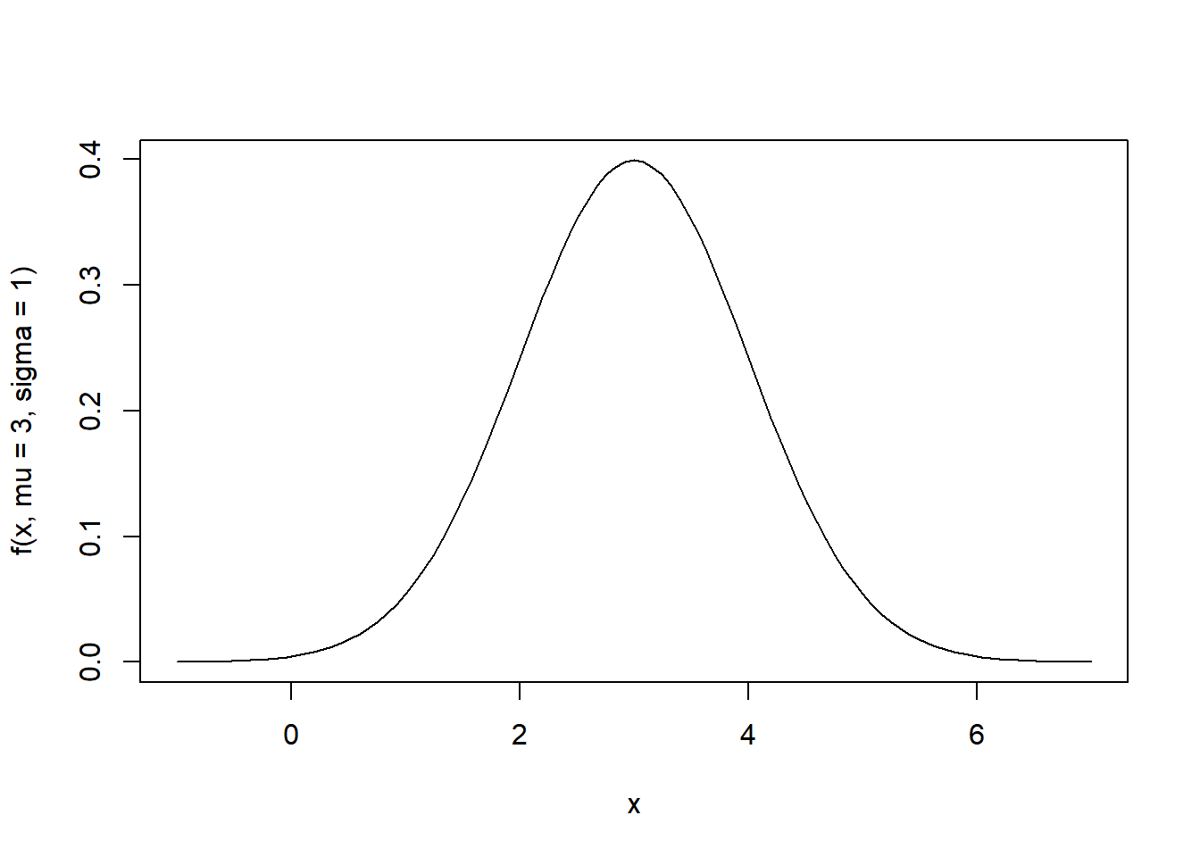

3.4.1.3 Predefined functions in R for PDF of a Normal

Question
Solution

Using the predefined function in R dnorm()⁴ to define the probability density function g as function of \(x\), \(mu\) and \(sigma\). Then plot g(x,0,1)

g <- function(x,mu,sigma) {
  dnorm(x,mean=mu,sd=sigma)
  }
curve(g(x,0,1), from = -3, to = 3)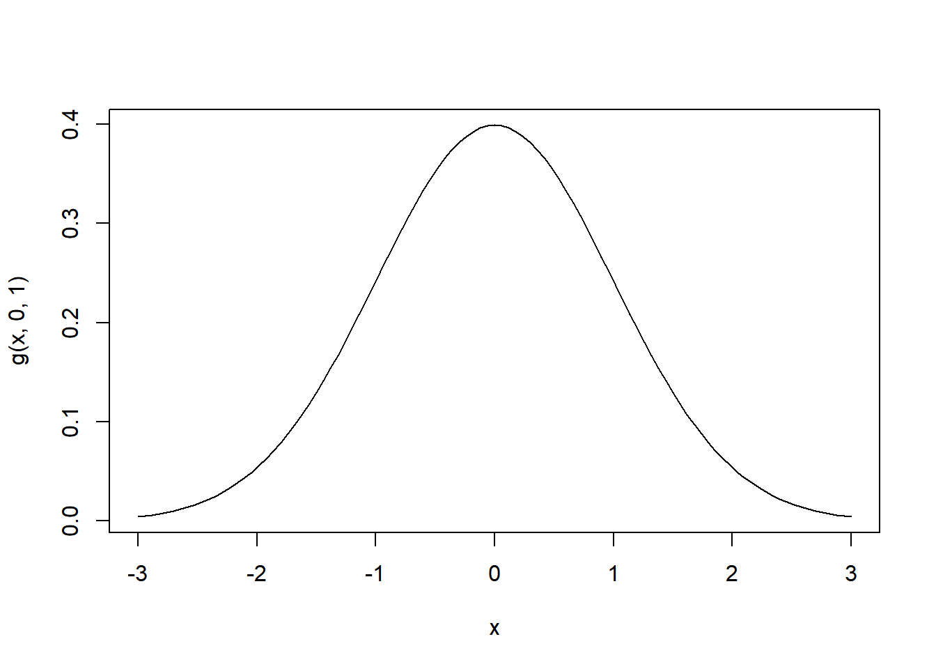

3.4.1.4 Predefined functions in R for CDF of a Normal

Question
Solution

Using the predefined function in R pnorm() to define the cumulative probability function cp as function of \(x\), \(mu\) and \(sigma\). Then plot cp(x,0,1)

cp <- function(x,mu,sigma) pnorm(x,mean=mu,sd=sigma)
curve(cp(x,0,1), from = -3, to = 3)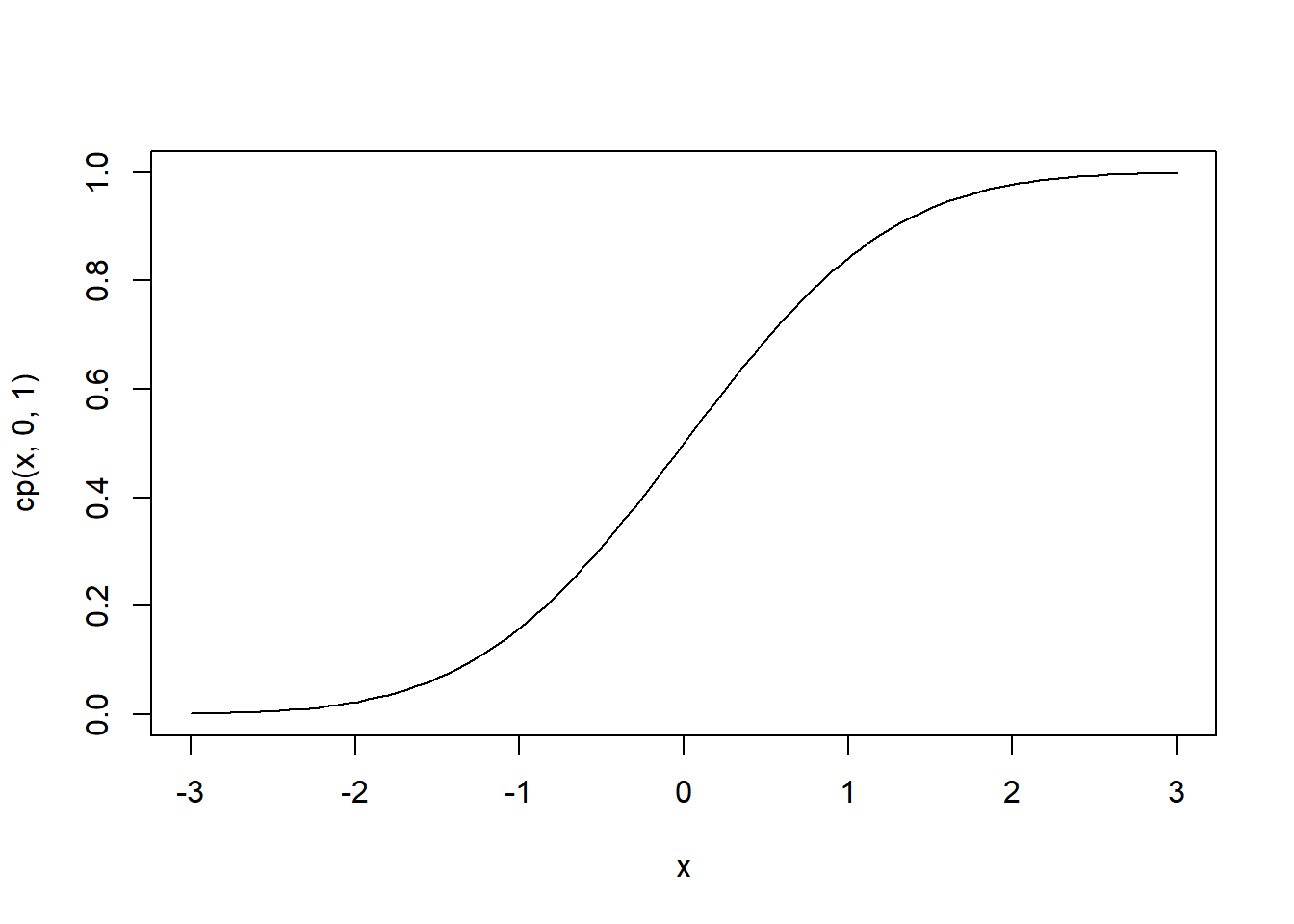

3.4.2 Areas and Probability

3.4.2.1 Estimating the probability

Question
Solution

By visual inspection of the plot of the last problem, estimate:

\(P(x<-2)\). The Probability for \(x<-2\).
\(P(x<0)\). The Probability for \(x<0\).
\(P(x<2)\). The Probability for \(x<2\).

The cumulative area under the curve seems negligible, therefore the probability is close to zero.
The cumulative area up to \(x=0\) is 0.5, or 50% of probability.
The cumulative probability from \(-\infty\) to \(x=2\) is a value very close to 1, that means is close to 100% but not equal.

3.4.2.2 Calculating the area⁵

Question
Solution

What is the probability of observing a value less than or equal to 0 in a standard normal distribution (X ~ N(0,1)), corresponding to the area under the curve from negative infinity to \(x = 0\)?

The area under the curve of a standard normal distribution, which has a mean (\(\mu\)) of 0 and a standard deviation (\(\sigma\)) of 1, from negative infinity (\(-\infty\)) to a specific value of x (in your case, x = 0) is equal to the cumulative distribution function (CDF) at that value of x.

For X ~ N(0,1), the CDF at x is given by:

\[ P(X \leq x) = \int_{-\infty}^{x} \frac{1}{\sqrt{2\pi}} e^{-\frac{t^2}{2}} dt \]

When x = 0, the area under the curve from negative infinity to 0 is:

\[ P(X \leq 0) = \int_{-\infty}^{0} \frac{1}{\sqrt{2\pi}} e^{-\frac{t^2}{2}} dt \]

This is the probability that a random draw from the standard normal distribution is less than or equal to 0, which can be calculated using statistical software, tables, or calculators. It turns out to be 0.5.

Easily compute this value using R:

# Calculate the prob: CDF P(X <= 0) for X ~ N(0,1)
probability <- pnorm(0, mean = 0, sd = 1)

# Print the result
paste("The probability is:", probability)

[1] "The probability is: 0.5"

Please note that the total area under the whole curve equals 1. When calculating the area from the far left to the central value, it amounts to 0.5. This result leverages the symmetry inherent in a normal distribution.

In summary, the probability of observing a value less than or equal to 0 in a standard normal distribution (X ~ N(0,1)) is 0.5. In the upcoming problems, I’ll provide concise solutions in the form of R code.

3.4.2.3 Calculating the probability

Question
Solution

Using the predefine function pnorm(), calculate:

\(P(x<-2)\). The Probability for \(x<-2\).
\(P(x<0)\). The Probability for \(x<0\).
\(P(x<2)\). The Probability for \(x<2\).

pnorm(q=-2,mean=0,sd=1)

[1] 0.02275013

pnorm(0,mean=0,sd=1)

[1] 0.5

pnorm(2,0,1) # parameters in order

[1] 0.9772499

3.4.2.4 Probability between x-scores.⁶

Assume \(X\) has a normal distribution with \(\mu =7\), and \(\sigma=3\), symbolically: \(X \sim N(7,3)\).

Calculate \(P(6<x<9)\)
Provide a visualization of the corresponding area to this probability.

\(P(6<x<9) = P(x<9) - P(x<6)\)

# Define the parameters
mu <- 7
sigma <- 3

# Calculate the probability P(6 < x < 9)
prob <- pnorm(9, mean = mu, sd = sigma) - pnorm(6, mean = mu, sd = sigma)

That means the probability of \(x\) to be between \(x=9\) and \(x=6\) is about 38%

# Load the ggplot2 library
library(ggplot2)

# Create a data frame for the density plot
df <- data.frame(x = seq(1, 12, length = 1000), 
                 y = dnorm(seq(1, 12, length = 1000), mean = mu, sd = sigma))

# Create the ggplot
plot <- ggplot(df, aes(x = x, y = y)) +
  geom_area(data = subset(df, x >= 6 & x <= 9), aes(y = y), fill = "lightblue") +
  geom_line() +
  labs(x = "X", y = "Density") +
  theme_minimal() +
  geom_vline(xintercept = c(6, 9), linetype = "dashed", color = "red") +
  annotate("text", x = 6.2, y = 0.07, label = paste("P(6 < x < 9) = ", round(prob, 2)), hjust = 0)

print(plot)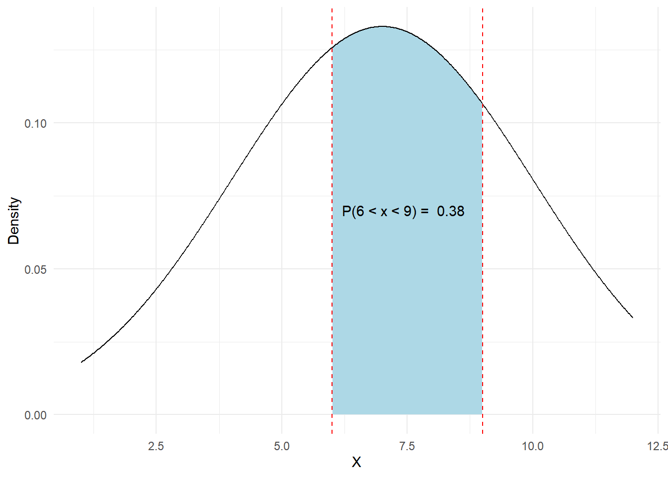

3.4.2.5 Probability between x-scores.

Question
Solution

Assume \(X\) has a normal distribution with \(\mu =100\), and \(\sigma=33\), symbolically: \(X \sim N(100,33)\).

Calculate:

The probability for \(x\) to be between 1 standard deviations from the center.
The probability for \(x\) to be between 2 standard deviations from the center.
The probability for \(x\) to be between 3 standard deviations from the center.

mu <- 100
sigma <- 33
pnorm(mu+sigma,mu,sigma)-pnorm(mu-sigma,mu,sigma)

[1] 0.6826895

pnorm(mu+2*sigma,mu,sigma)-pnorm(mu-2*sigma,mu,sigma)

[1] 0.9544997

pnorm(mu+3*sigma,mu,sigma)-pnorm(mu-3*sigma,mu,sigma)

[1] 0.9973002

3.4.3 Scores and Critical Values

Definition

A \(z-score\) is a convenient measure of how far, in standard deviation units, the score is from the center.

If \(X\) is a normally distributed random variable and \(X\sim N(\mu,\sigma)\), then the z-score⁷ is:

\[\boxed{z=\frac{x-\mu}{\sigma}}\] Solving for \(x\):

\[x = z\sigma+\mu\] Note: A standard normal distribution variable \(Z\), implies that \(\mu=0\) and \(\sigma=1\). \(Z\sim N(0,1)\)

3.4.3.1 z-score function in R

Question
Solution

Create a function in R that calculate z-scores:

z_score <- function(x,mu,sigma) {
  (x-mu)/sigma 
  }

3.4.3.2 Calculate the z-score

Question
Solution

What is the z-score for the value \(x = 18\) in a normally distributed variable \(X\) with a mean of 12 and a standard deviation of 3?

z_score(x=18,mu=12,sigma=3)

[1] 2

#OR
z_score(18,12,3) # parameters in order of definition

[1] 2

3.4.3.3 Calculate the z-score

Question
Solution

Max averages 33 points per game with a standard deviation of 5 points, represented as \(X\sim N(33,5)\). If Max scores 40 points in the last game, what is the corresponding z-score for that game?

z_score(40,33,5)

[1] 1.4

3.4.3.4 Calculate the z-score

Question
Solution

Some doctors believe that a person can lose 8 pounds, on average, in a month by reducing their fat intake and exercising consistently. Suppose weight loss follows a normal distribution. Let \(X\) be the amount of weight lost (in pounds) by a person in a month. Using a standard deviation of 4 pounds, calculate the z-score for a person losing 5 pounds.

[1] "x =  5"

[1] "mean =  8"

[1] "sigma =  4"

[1] "The z-score =  -0.75"

3.4.3.5 Calculate the z-score using `scale()` function.

Question
Solution

The scores on a standardized math test are normally distributed with a mean (μ) of 75 and a standard deviation (σ) of 10. Sarah scored 85 on the test. Calculate the z-score for Sarah’s score.

scale(x=85,center=75,scale=10)

     [,1]
[1,]    1
attr(,"scaled:center")
[1] 75
attr(,"scaled:scale")
[1] 10

3.4.3.6 Calculate the z-score for a list of numbers.

Calculate the z-scores for the following list of numbers: \[\{1,2,3,4,5,6,7\}\]
What is the mean and standard deviation of the previous list?

x <- c(1,2,3,4,5,6,7)
zs <- scale(x)
zs

           [,1]
[1,] -1.3887301
[2,] -0.9258201
[3,] -0.4629100
[4,]  0.0000000
[5,]  0.4629100
[6,]  0.9258201
[7,]  1.3887301
attr(,"scaled:center")
[1] 4
attr(,"scaled:scale")
[1] 2.160247

By observing the attributes of the output of the scale function we can said that the mean of the list is 4 and the standard deviation is 2.16. We can check using mean() and sd() functions:

mean(x)

[1] 4

sd(x)

[1] 2.160247

3.4.3.7 Calculate an x-score

Question
Solution

Suppose \(X\sim N(2,6)\). What value of \(x\) has a z-score of three?

x_score <- function(z,sigma,mu) { z*sigma +mu }
x_score(3,6,2)

[1] 20

3.4.3.8 Calculate an x-score

Question
Solution

Suppose \(X\sim N(8,1)\). What value of \(x\) has a z-score of -2.25?

x_score(sigma=1,mu=8, z=-2.25)

[1] 5.75

Note: Please note that on this last example we have intentionally provided the values of the parameters in a different order than what was the definition of our x_score function. This is permissible as long as we provide the names of the parameters. If no names are provided, the function should be called as x_score(-2.25, 1, 8).

3.4.4 Level of significance

Definition

The level of significance in statistics, often denoted by \(\alpha\), is a threshold used to determine whether a result is statistically significant. It represents the probability of rejecting a true null hypothesis, also known as a Type I error.

3.4.5 Rejection Zone

Definition

When a specific level of significance is established, such as \(\alpha=0.05\), the rejection zone refers to the regions located in the tails of the distribution, collectively accounting for 5% of the total area under the curve. This area represents the range of values for which, if the test statistic falls within, we would reject the null hypothesis. By doing so, we acknowledge that observing such extreme values is unlikely (with a probability of 5% or less) if the null hypothesis were true. Therefore, the rejection zone is crucial in determining the threshold for statistical significance in hypothesis testing. We will dive deeper on hypothesis testing on a future chapter.

Warning in geom_point(aes(x = -critical_value, y = 0), color = "black", : All aesthetics have length 1, but the data has 601 rows.
ℹ Please consider using `annotate()` or provide this layer with data containing
  a single row.

Warning in geom_point(aes(x = critical_value, y = 0), color = "black", size = 3, : All aesthetics have length 1, but the data has 601 rows.
ℹ Please consider using `annotate()` or provide this layer with data containing
  a single row.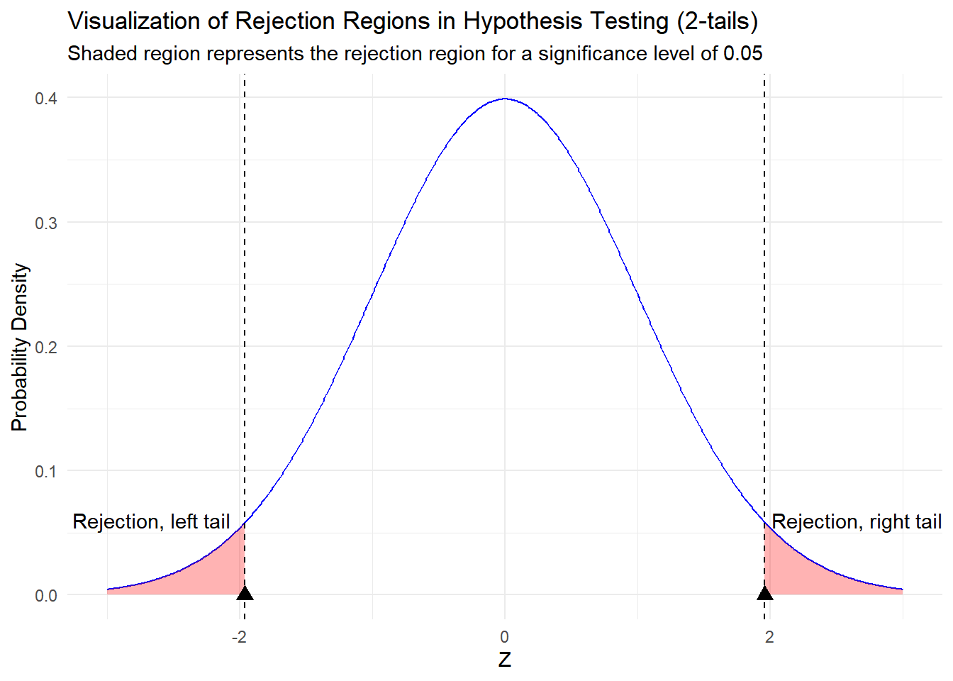

3.4.6 Statistically significant

Informal definition

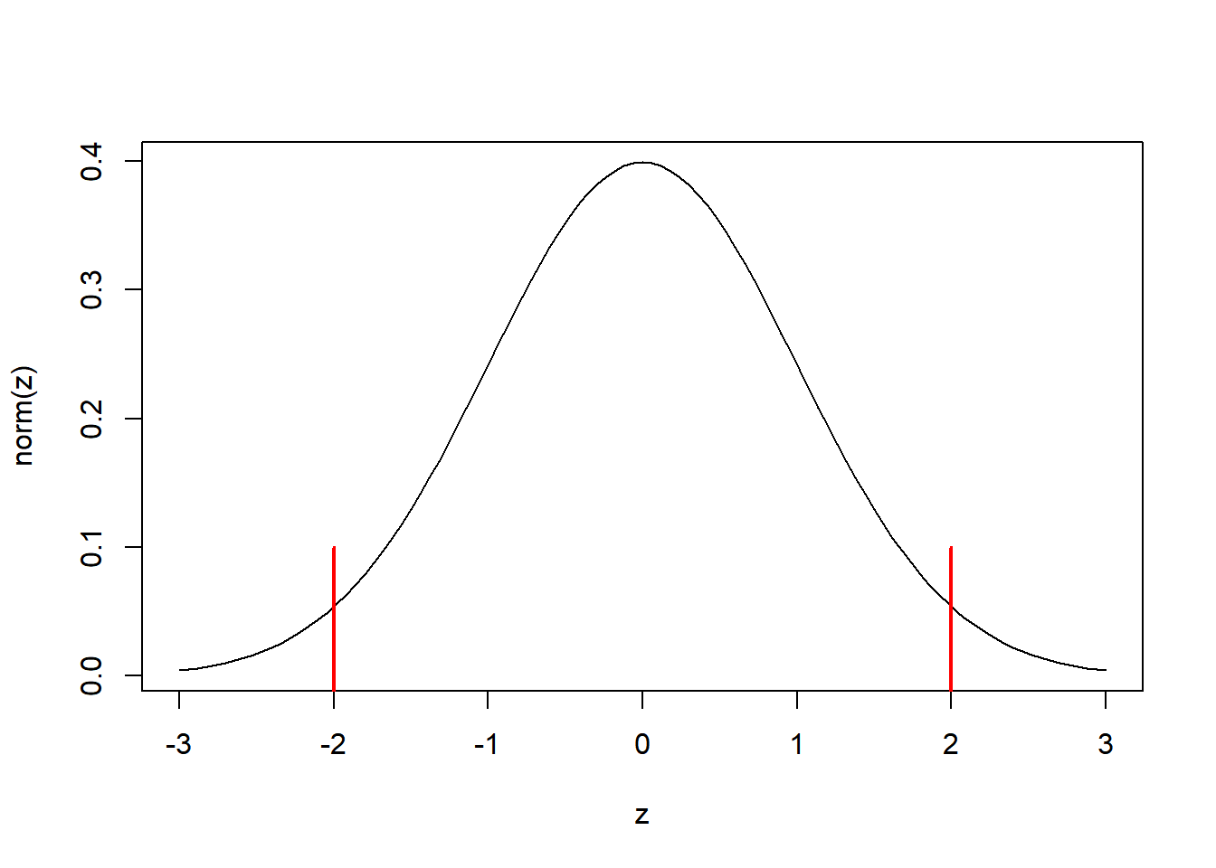
When a z-score falls within the rejection region, we deem the statistic as ‘statistically significant.’ In the context of normal distributions, a commonly employed rule of thumb is that the rejection region spans approximately two standard deviations to the left and two standard deviations to the right of the distribution’s center. This means that extreme values in either direction from the mean are considered statistically significant, indicating the presence of an effect or difference from what would be expected under the null hypothesis.

Example 1

Question
Solution

State if \(x=20\) is statistically significant or not. \(X\sim N(18,1.1)\)

scale(20,center=18,scale=1.1)

         [,1]
[1,] 1.818182
attr(,"scaled:center")
[1] 18
attr(,"scaled:scale")
[1] 1.1

Because the absolute value of the z-score is less than 2, then is not statistically significant. (\(\alpha=0.05\))

Example 2

Question
Solution

Max averages 33 points a game with a standard deviation of 5 points. \(X\sim N(33,5)\). Suppose Max scores 44 points in the last game, is this game out of the ordinary? Statistically Significant? Justify your answer.

We can calculate the \(z-score\) using the scale() function:

scale(44,center=33,scale=5)

     [,1]
[1,]  2.2
attr(,"scaled:center")
[1] 33
attr(,"scaled:scale")
[1] 5

Our calculated \(z-score\) exceeds 2. Interpreting this result in the context of a 0.05 level of significance (\(\alpha=0.05\)), we can assert that the game’s outcome is statistically significant. Go Max! ^^

Example 3, exhaustive explanation.

Question
Solution

Jack regularly goes fishing, and he typically catches an average of 12 fish per trip with a standard deviation of 3 fish. On his last fishing trip, he caught 18 fish. Is this fishing trip out of the ordinary? Statistically Significant? Justify your answer.

To determine if Jack’s last fishing trip is out of the ordinary or statistically significant, we can calculate the z-score for the number of fish he caught, which is 18, using the given information.

The formula for calculating the z-score is:

\[Z = \frac{X - \mu}{\sigma}\]

Where: - \(X\) is the value of interest (the number of fish Jack caught), which is 18. - \(\mu\) is the population mean, which is his average catch, 12 fish. - \(\sigma\) is the population standard deviation, 3 fish.

Substitute these values into the formula:

\[Z = \frac{18 - 12}{3} = \frac{6}{3} = 2\]

Now, let’s interpret the z-score. A z-score of 2 indicates that Jack’s catch of 18 fish is 2 standard deviations above his average. In the context of fishing, a z-score of 2 suggests that his catch of 18 fish is quite unusual and statistically significant. It’s significantly higher than what he typically catches.

Using R:

scale(18,12,3)

     [,1]
[1,]    2
attr(,"scaled:center")
[1] 12
attr(,"scaled:scale")
[1] 3

Because \(z-score=2\) fall barely on the rejection zone, we do consider this fishing trip out of the ordinary.

3.4.7 p-value

The p-value, is the probability of observing a value as extreme as, or more extreme than, a specific observed value. In other words, it quantifies the likelihood of obtaining such an extreme result by chance.

When you calculate a p-value, you’re essentially finding the area under the normal distribution curve in the tail(s) that corresponds to values at least as extreme as the one you’ve observed. A smaller p-value indicates that the observed value is in a less probable region of the distribution.

If the p-value is less than or equal to the level of significance (alpha), the observed data provides sufficient evidence to conclude that the statistic results did not happen by chance.

Example

Question
Solution

Max averages 33 points a game with a standard deviation of 5 points. \(X\sim N(33,5)\). Suppose Max scores 44 points in the last game, what is p-value associated with this score?

We can calculate the \(z-score\) using the scale() function:

mu <- 33
sigma <- 5
z_score <- as.numeric(scale(44,mu,sigma))
z_score

[1] 2.2

Now the \(p-value\) is found in the area on the right tail, because the score is at the right of the center:

p_value <- 1-pnorm(z_score, 0, 1)
p_value

[1] 0.01390345

#OR Directly from the x-score
p_value <- 1-pnorm(44,33, 5)
p_value

[1] 0.01390345

#OR
p_value <- pnorm(44,33, 5, lower.tail = FALSE)
p_value

[1] 0.01390345

That means that the likelihood that Max obtain this result by chance is so small ( ~ 1%), that we should support the claim that Max did a game out of the ordinary!

3.5 Normal Problems

3.5.1

Question
Solution

A normal distribution has a mean of 61 and a standard deviation of 15. What is the median?

In a normal distribution, the median is equal to the mean, which is 61 in this case. The median of a normal distribution is always at the center of the distribution, and the mean also represents the center of the distribution for a symmetric bell-shaped curve like the normal distribution.

3.5.2

Question
Solution

Suppose the random variables X and Y have the following normal distributions: X ~ N(5, 6) and Y ~ N(2, 1). If x = 17, then z = 2. If y = 4, what is z?

z <- scale(4,2,1)
print(z)

     [,1]
[1,]    2
attr(,"scaled:center")
[1] 2
attr(,"scaled:scale")
[1] 1

3.5.3

Jerome averages 16 points per game with a standard deviation of four points. X ~ N(16,4). Suppose Jerome scores ten points in the last game.

What is the z-score for the last game?
How many standard deviations far from the center is the z-score? To the left or to the right?
Is this game out of the ordinary?

scale(10,16,4)

     [,1]
[1,] -1.5
attr(,"scaled:center")
[1] 16
attr(,"scaled:scale")
[1] 4

1.5 standard deviations to the left of the mean.

Is not statistically significant, because the z-score is inside of 2 standard deviations from the center.

3.5.4

Question
Solution

Considering that the height of 15 to 18-year-old males from Chile in the years 2009 to 2010 follows a normal distribution with a mean of 170 cm and a standard deviation of 6.28 cm, we can represent this with the notation X ~ N(170, 6.28). Given this distribution, how statistically unusual is it to observe a Chilean male in this age group with a height of 185 cm?

scale(185,170,6.28)

         [,1]
[1,] 2.388535
attr(,"scaled:center")
[1] 170
attr(,"scaled:scale")
[1] 6.28

A Chilean male with a height of 185 cm is statistically unusual, because the z-score is about 2.39 standard deviations above the mean. (\(\alpha = 0.05\))

3.5.5

The final exam scores in a statistics class were normally distributed with a mean of 63 and a standard deviation of five.

Find the probability that a randomly selected student scored more than 65 on the exam.
Find the probability that a randomly selected student scored less than 85.
Find the 90th percentile (that is, find the score k that has 90% of the scores below k and 10% of the scores above k).

\(P(x>65) = 1 - P(x<65)\):

probability <- 1 - pnorm(65, mean = 63, sd = 5) 
#OR
probability <- pnorm(65, mean = 63, sd = 5, lower.tail = FALSE)
paste("The probability is:", round(100*probability,3),"%")

[1] "The probability is: 34.458 %"

\(P(x<85)\):

probability <- pnorm(85, mean = 63, sd = 5)
paste("The probability is:", round(100*probability,3),"%")

[1] "The probability is: 99.999 %"

We need to find \(k\) which satisfy \(P(x<k)=0.90\):

quartile <- qnorm(.90, mean = 63, sd = 5)
paste("The 90th percentile is found at the score k =", round(quartile,1))

[1] "The 90th percentile is found at the score k = 69.4"

3.5.6

Question
Solution

3.7 List of Machine Learning Algorithms

Many machine learning algorithms make the assumption that the input data is normally distributed⁸, or they perform better when the data conforms to a normal distribution. However, it’s important to note that this doesn’t mean these algorithms strictly require normally distributed data; they can often still perform reasonably well on non-normal data, especially if the sample size is large enough due to the Central Limit Theorem.

Here is a list of some algorithms that often benefit from normally distributed data:

Linear Regression: Assumes that the residuals (differences between the predicted and actual values) are normally distributed.
Logistic Regression: Works better if the predictors are roughly normally distributed, especially for small sample sizes.
Linear Discriminant Analysis (LDA): Assumes that the features are normally distributed and have the same covariance matrix for each class.
Principal Component Analysis (PCA): Works best if the data is normally distributed, as it relies on estimating the covariance matrix.
Gaussian Naive Bayes: Assumes that the likelihood of the features is Gaussian.
Parametric Statistical Tests: Such as t-tests and ANOVAs, which assume that the samples are drawn from normally distributed populations.
Support Vector Machines (SVMs) with certain kernels: Performance can be influenced by the distribution of the data.
Pearson’s Correlation Coefficient: Assumes that the two variables being compared are normally distributed.
Multivariate Analysis: Such as MANOVA, which assumes multivariate normality.
Ridge and Lasso Regression: These linear models can benefit from normally distributed data.
k-Means Clustering: While not explicitly requiring normality, it assumes that the clusters are spherical and equally sized, which is more likely if the data is normally distributed.
Neural Networks: Although they are quite flexible and can handle non-normal data, their performance might be improved if the inputs are scaled and normalized.
General Linear Models (GLMs): Assume that the residuals are normally distributed.
Q-Q Plots and Other Normality Tests: Used explicitly to check if a dataset is normally distributed.

It is important to apply the necessary transformations or select appropriate algorithms based on the distribution of your data. In practice, normalizing the data (e.g., using z-score normalization) or transforming it to a more normal distribution (e.g., using a log or Box-Cox transformation) can sometimes improve the performance of these algorithms if the data is not already normally distributed.

References and footnotes

Gauss, C. (2011). THEORIA MOTUS CORPORUM COELESTIUM IN SECTIONIBUS CONICIS SOLEM AMBIENTIUM. In E. Schering (Ed.), Werke (Cambridge Library Collection - Mathematics, pp. 1-2). Cambridge: Cambridge University Press. doi:10.1017/CBO9781139058285.001↩︎
Author: OpenAI. (2023, June 8). “What is the definition for a normally distributed variable?” (Version 1). ChatGPT. https://www.openai.com↩︎
Author: OpenAI. (2023, October 31). “R Functions for Normal Distributions” (Version 1). ChatGPT. https://www.openai.com↩︎
rdocumentation.org, package: stats, functions: dnorm(), pnorm(). https://www.rdocumentation.org/packages/stats/versions/3.6.2/topics/Normal ↩︎
Tutorial, don’t skip this problem.↩︎
Great Code for Visualization of areas.↩︎
The z-score tells you how many standard deviations the value \(x\) is above (to the right of) or below (to the left of) the mean (\(\mu\))↩︎
Author: OpenAI. (2023, October 31). “ML Algorithms and normal distribution.” ChatGPT. https://www.openai.com↩︎

3.1 Introduction to the Gaussian distribution

3.2 The Mathematics

3.3 Functions in R

3.3.1 Functions for Probability and Areas:

3.3.2 Functions for Z-Scores:

3.3.3 Normality Tests:

3.4 Basic Problems

3.4.1 Normal definitions and plots

3.4.1.1 Define a Normal function in R

3.4.1.2 Plot the PDF for a normal

3.4.1.3 Predefined functions in R for PDF of a Normal

3.4.1.4 Predefined functions in R for CDF of a Normal

3.4.2 Areas and Probability

3.4.2.1 Estimating the probability

3.4.2.2 Calculating the area5

3.4.2.3 Calculating the probability

3.4.2.4 Probability between x-scores.6

3.4.2.5 Probability between x-scores.

3.4.3 Scores and Critical Values

3.4.3.1 z-score function in R

3.4.3.2 Calculate the z-score

3.4.3.3 Calculate the z-score

3.4.3.4 Calculate the z-score

3.4.3.5 Calculate the z-score using scale() function.

3.4.3.6 Calculate the z-score for a list of numbers.

3.4.3.7 Calculate an x-score

3.4.3.8 Calculate an x-score

3.4.4 Level of significance

3.4.5 Rejection Zone

3.4.6 Statistically significant

3.4.7 p-value

3.5 Normal Problems

3.5.1

3.5.2

3.5.3

3.5.4

3.5.5

3.5.6

3.6 Statistical Significant Problems

3.6.1

3.6.2

3.6.3

3.6.4

3.6.5

3.6.6

3.6.7

3.6.8

3.6.9

3.6.10

3.6.11

3.6.12

3.7 List of Machine Learning Algorithms

References and footnotes

3.1 Introduction to the `Gaussian` distribution

3.4.2.2 Calculating the area⁵

3.4.2.4 Probability between x-scores.⁶

3.4.3.5 Calculate the z-score using `scale()` function.