Non-normal distributions1 encompass a wide range of statistical distributions that deviate from the characteristics of a normal distribution. While a normal distribution is symmetric and bell-shaped, non-normal distributions can exhibit various shapes, asymmetry, and differing tail behavior. Understanding and identifying non-normal distributions is crucial in statistics because many statistical tests and models assume normality or make specific assumptions about the underlying distribution of the data.
Here are some common types of non-normal distributions:
Skewed Distributions:
Positively Skewed (Right Skewed): In a positively skewed distribution, the tail extends towards the right, indicating a concentration of lower values. The mean is typically greater than the median.
Negatively Skewed (Left Skewed): In a negatively skewed distribution, the tail extends towards the left, indicating a concentration of higher values. The mean is typically less than the median.
Uniform Distribution:
A uniform distribution is characterized by a constant probability density function over a specific range. It represents a situation where all values within the range have an equal likelihood of occurring, resulting in a flat and constant shape.
Bimodal and Multimodal Distributions:
Bimodal Distribution: A bimodal distribution has two distinct peaks or modes, indicating the presence of two separate groups or subpopulations within the data. Each mode represents a different set of characteristic values.
Multimodal Distribution: A multimodal distribution has more than two distinct peaks, indicating the presence of multiple subpopulations or groups with different characteristic values.
Exponential Distribution:
An exponential distribution is characterized by a continuous probability density function that rapidly decreases as the value increases. It is commonly used to model events that occur randomly over time, such as the time between successive events in a Poisson process.
Log-Normal Distribution:
The log-normal distribution is a skewed distribution where the logarithm of the data follows a normal distribution. It often arises when data is generated by a multiplicative process, resulting in a positively skewed distribution of the original values.
Weibull Distribution:
The Weibull distribution is a flexible distribution that can exhibit a range of shapes, including positively skewed, negatively skewed, and symmetric distributions. It is commonly used to model reliability, survival, and failure times.
Pareto Distribution:
The Pareto distribution is a heavy-tailed distribution that is often used to model phenomena where a small number of extreme events have a significant impact compared to the majority of more common events. It is characterized by a power-law relationship between the variables.
These are just a few examples of non-normal distributions encountered in statistics. It is essential to identify the appropriate distribution for a given dataset to ensure accurate analysis, model selection, and inference. Statistical techniques and tests exist to analyze data that do not follow a normal distribution, allowing researchers to make valid conclusions even with non-normal data.
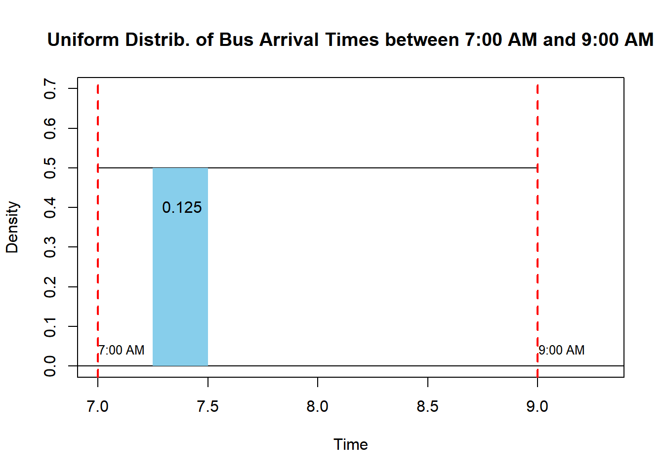
You are investigating the arrival times of buses at a particular bus stop. The arrival times are assumed to follow a uniform distribution between 7:00 AM and 9:00 AM.
Probability Calculation:
Calculate the probability that a bus arrives between 7:15 AM and 7:30 AM.
Percentile Calculation:
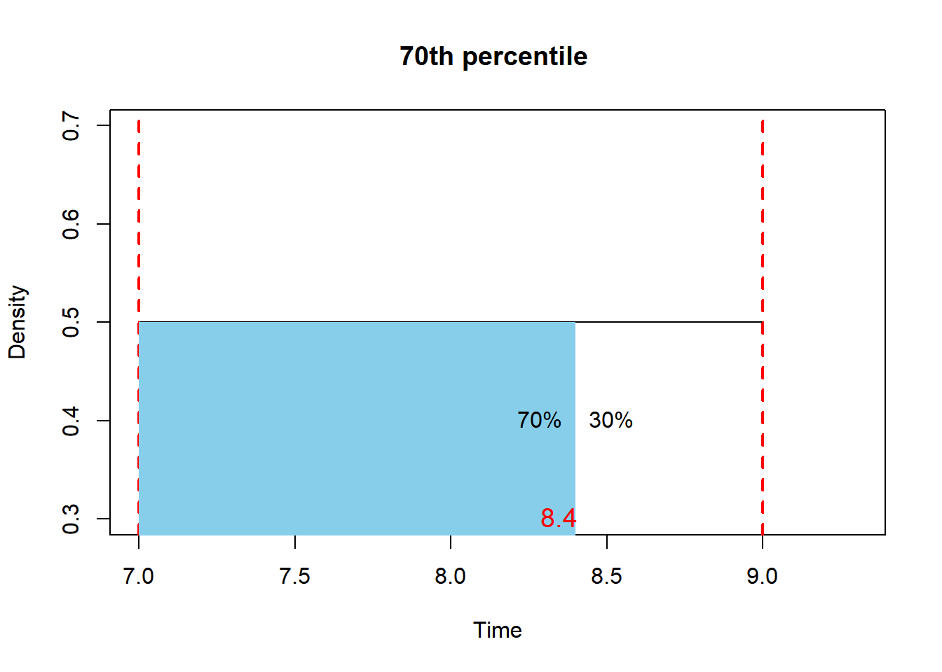
Determine the 70th percentile of the arrival times distribution.
Provide visualizations.
Problem: Calculate the probability that a bus arrives between 7:15 AM and 7:30 AM.
Solution:
In a probability density function (PDF), the total area under the curve must sum up to 1. For a uniform distribution, where the arrival time spans between 7 AM to 9 AM, the height of this PDF should be 1/2, ensuring that the total area equals 1.
# Parametersstart_time <-7# 7:00 AM in decimal formatend_time <-9# 9:00 AM in decimal formatshade_start <-7.25# 7:15 AM in decimal formatshade_end <-7.5# 7:30 AM in decimal format# Vectors for the PDFx <-seq(start_time, end_time, length.out =1000)y <-dunif(x, min = start_time, max = end_time)# Plotting the uniform distribution and additional linesplot(x, y, type ="l", xlim =c(7,9.3), ylim=c(0,0.7),xlab ="Time", ylab ="Density", main ="Uniform Distrib. of Bus Arrival Times between 7:00 AM and 9:00 AM")abline(v =c(start_time, end_time), col ="red", lty =2, lwd =2)abline(h =0, col ="black", lty =1, lwd =1)# Shading the area between 7:15 AM and 7:30 AMshade_x <-c(shade_start, seq(shade_start, shade_end, length.out =100), shade_end)shade_y <-c(0, dunif(seq(shade_start, shade_end, length.out =100), min = start_time, max = end_time), 0)polygon(shade_x, shade_y, col ="skyblue", border =NA)# Annotations for the probability and visual aidstext(7.25, 0.4, paste(1/2*(7.5-7.25)), pos =4)text(start_time-0.04, 0.04, "7:00 AM", pos =4,cex=0.8)text(end_time-0.04, 0.04, "9:00 AM", pos =4,cex=0.8)
This code segment produces a plot illustrating the uniform distribution of bus arrival times between 7:00 AM and 9:00 AM, with a shaded area representing the specific time range. Additionally, it includes annotations indicating the probability calculation and the time notations aligned with the plot for clarity
Problem: Determine the 70th percentile of the arrival times distribution.
Solution:
We aim to determine the value of x that separates 70% of the accumulated area from the remaining 30% in our uniform distribution. This entails solving the equation:
\(0.7 = (x-7)*1/2\)
# Define the equationequation <-function(x) { (x -7) * (1/2) -0.7}# Use a root-finding function (e.g., uniroot) to solve the equationsolution <-uniroot(equation, c(0, 20)) # Adjust the range [0, 20] as needed# Extract the value of x from the solutionx_value <- solution$rootx_value
[1] 8.4
# Parametersstart_time <-7# 7:00 AM in decimal formatend_time <-9# 9:00 AM in decimal formatshade_start <-7# 7:15 AM in decimal formatshade_end <-8.4# 7:30 AM in decimal format# Plotting the uniform distribution with shading and annotationx <-seq(start_time, end_time, length.out =1000)y <-dunif(x, min = start_time, max = end_time)plot(x, y, type ="l", xlim =c(7,9.3),xlab ="Time", ylab ="Density", main ="70th percentile ")abline(v =c(start_time, end_time), col ="red", lty =2, lwd =2)# Shading the area between 7:15 AM and 7:30 AMshade_x <-c(shade_start, seq(shade_start, shade_end, length.out =100), shade_end)shade_y <-c(0, dunif(seq(shade_start, shade_end, length.out =100), min = start_time, max = end_time), 0)polygon(shade_x, shade_y, col ="skyblue", border =NA)# Annotation for the percentiletext(8.4, 0.4, "70%", pos =2)text(8.4, 0.4, "30%", pos =4)text(8.45, 0.3, "8.4", pos =2, cex=1.2, col ="red")
Description: To find a percentile in a uniform distribution, the difference between the start and end points of the interval is scaled according to the desired percentile value.
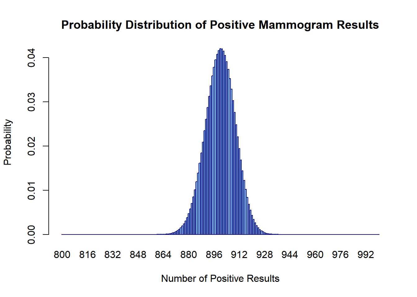
You are a medical researcher investigating the accuracy of a breast cancer screening mammogram. The mammogram has a reported accuracy of 90%, meaning that if a patient has breast cancer, there is a 90% chance the mammogram will correctly detect it. You have a group of 1,000 women undergoing mammograms. Calculate the following probabilities using R:
What is the probability that exactly 950 out of 1,000 women will receive a positive mammogram result?
What is the probability that fewer than 100 women will receive a positive mammogram result?
What is the probability that more than 900 women will receive a positive mammogram result?
Visualize the probability distribution for the number of positive mammogram results in the 1,000 women undergoing mammograms.
Probability of exactly 950 out of 1,000 women getting a positive result:
# Generate probabilities for different numbers of positive resultsn <-1000prob <-dbinom(800:1000, size = n, prob =0.9)# Create a bar plotbarplot(prob, names.arg =800:1000, xlab ="Number of Positive Results", ylab ="Probability", main ="Probability Distribution of Positive Mammogram Results",col ='skyblue', border ='darkblue')
A goat cheese manufacturing process involves pasteurizing milk, and the time (in minutes) required for pasteurization follows a t-student distribution with 20 degrees of freedom.
Probability Calculation:
Calculate the probability that the pasteurization time is less than 25 minutes.
Percentile Calculation:
Determine the 80th percentile of the pasteurization time distribution.
Hypothesis Testing:
The cheese producer claims that the average pasteurization time is 30 minutes. Conduct a hypothesis test at a 5% significance level to determine if there is enough evidence to reject this claim based on a sample of 15 pasteurization time measurements, where the sample mean is 28 minutes, and the sample standard deviation is 5 minutes.
Confidence Interval:
Calculate a 95% confidence interval for the average pasteurization time based on a sample of 20 pasteurization time measurements, where the sample mean is 32 minutes, and the sample standard deviation is 6 minutes.
Problem: Calculate the probability that the pasteurization time is less than 25 minutes.
\[P(X<25)\]
Solution:
# Parametersdf <-20# degrees of freedom# Probability calculationprob_less_than_25 <-pt(25, df)prob_less_than_25
[1] 1
Description: The pt function is used to calculate the cumulative probability (CDF) for a t-student distribution. The result represents the probability that the pasteurization time is less than 25 minutes.
Problem: Determine the 80th percentile of the pasteurization time distribution.
Description: The qt function is employed to find the quantile (inverse CDF) for a t-student distribution. The result represents the 80th percentile of the pasteurization time distribution.
Problem: The cheese producer claims that the average pasteurization time is 30 minutes. Conduct a hypothesis test at a 5% significance level to determine if there is enough evidence to reject this claim based on a sample of 15 pasteurization time measurements, where the sample mean is 28 minutes, and the sample standard deviation is 5 minutes.
Description: The t-statistic and p-value are calculated using the provided sample information. The null hypothesis is tested against the claim mean, and the result indicates whether there is enough evidence to reject the producer’s claim.
Problem: Calculate a 95% confidence interval for the average pasteurization time based on a sample of 20 pasteurization time measurements, where the sample mean is 32 minutes, and the sample standard deviation is 6 minutes.
Description: The margin of error is calculated based on the t-distribution, and a confidence interval is constructed around the sample mean. The result provides a range within which we can be 95% confident that the true average pasteurization time lies.
These R code snippets provide the solutions to each part of the quiz problem, demonstrating how to perform probability calculations, percentiles, hypothesis testing, and confidence intervals using a t-student distribution.
You are a researcher investigating the distribution of vehicle types in a city’s downtown area. After conducting a survey, you find that the observed distribution differs from the expected distribution based on national statistics.
Goodness-of-Fit Test:
Perform a goodness-of-fit chi-square test at a 1% significance level to assess whether the observed distribution matches the expected distribution. Use the following data:
Vehicle Type
Observed Frequency
Expected Frequency
Car
120
100
Motorcycle
40
30
Bicycle
30
20
Pedestrian
50
60
Independence Test:
Conduct a chi-square test for independence to determine if there is a significant association between vehicle type and time of day. Use the following contingency table:
Morning
Afternoon
Evening
Car
50
40
30
Motorcycle
10
20
10
Bicycle
20
10
5
Pedestrian
40
30
20
Perform the test at a 5% significance level.
Confidence Interval:
Calculate a 90% confidence interval for the expected frequency of bicycles based on national statistics. The observed frequency of bicycles in the downtown area is 30.
Problem: Perform a goodness-of-fit chi-square test at a 1% significance level to assess whether the observed distribution matches the expected distribution.
Description: The chisq.test function is used to perform a goodness-of-fit chi-square test. The p-value is checked against the significance level to determine if there is a significant difference between the observed and expected distributions.
Problem: Conduct a chi-square test for independence to determine if there is a significant association between vehicle type and time of day.
Description: The chisq.test function is employed to perform a chi-square test for independence. The p-value is checked against the significance level to determine if there is a significant association between vehicle type and time of day.
Problem: Calculate a 90% confidence interval for the expected frequency of bicycles based on national statistics. The observed frequency of bicycles in the downtown area is 30.
Description: The prop.test function is used to calculate a confidence interval for the expected frequency of bicycles based on the chi-square distribution. The result provides a range within which we can be 90% confident that the true expected frequency of bicycles lies.
In a quality control process, the variation in the diameters of two types of components is being compared. The diameters of Type A components follow an F-distribution with 3 and 15 degrees of freedom, and the diameters of Type B components follow an F-distribution with 5 and 20 degrees of freedom.
Probability Calculation:
Calculate the probability that the diameter ratio (Type A diameter divided by Type B diameter) is less than 2.
Percentile Calculation:
Determine the 90th percentile of the diameter ratio.
Description: The pf function is used to calculate the cumulative probability (CDF) for an F-distribution. The result represents the probability that the diameter ratio is less than 2.
Description: The qf function is employed to find the quantile (inverse CDF) for an F-distribution. The result represents the 90th percentile of the diameter ratio.
In a coffee shop, the number of customers entering per hour follows a Poisson distribution with an average rate of 10 customers per hour.
Probability Calculation:
Calculate the probability of having exactly 7 customers entering the coffee shop in a given hour.
Percentile Calculation:
Determine the 75th percentile of the number of incoming customers per hour.
Hypothesis Testing:
The coffee shop manager claims that the average customer rate is 12 customers per hour. Conduct a hypothesis test at a 5% significance level based on a sample of 8 hours, where the observed average customer rate is 11 customers per hour.
Confidence Interval:
Calculate a 90% confidence interval for the average customer rate based on a sample of 12 hours, where the observed average customer rate is 9 customers per hour.
Certainly! Here’s the detailed description and R code for each part of the revised quiz problem:
Problem: Calculate the probability of having exactly 7 customers entering the coffee shop in a given hour.
Solution:
# Parametersaverage_rate <-10number_of_customers <-7# Probability calculationprob_exactly_7_customers <-dpois(number_of_customers, lambda = average_rate)prob_exactly_7_customers
[1] 0.09007923
Description: The dpois function is used to calculate the probability of a specific number of events occurring in a Poisson distribution. The result represents the probability of having exactly 7 customers entering the coffee shop in a given hour.
Problem: Determine the 75th percentile of the number of incoming customers per hour.
Description: The qpois function is employed to find the quantile (inverse CDF) for a Poisson distribution. The result represents the 75th percentile of the number of incoming customers per hour.
Problem: The coffee shop manager claims that the average customer rate is 12 customers per hour. Conduct a hypothesis test at a 5% significance level based on a sample of 8 hours, where the observed average customer rate is 11 customers per hour.
Description: The poisson.test function is used to perform a hypothesis test for a Poisson distribution. The p-value is checked against the significance level to determine if there is enough evidence to reject the manager’s claim.
Problem: Calculate a 90% confidence interval for the average customer rate based on a sample of 12 hours, where the observed average customer rate is 9 customers per hour.
Description: The poisson.test function is used to calculate a confidence interval for the average customer rate based on a Poisson distribution. The result provides a range within which we can be 90% confident that the true average customer rate lies.
In a web server, the time (in minutes) between consecutive requests follows an exponential distribution with an average rate of 0.2 requests per minute.
Probability Calculation:
Calculate the probability that the time between consecutive requests is less than 5 minutes.
Percentile Calculation:
Determine the 80th percentile of the time between consecutive requests.
Hypothesis Testing:
The server administrator claims that the average time between consecutive requests is 6 minutes. Conduct a hypothesis test at a 1% significance level based on a sample of 15 time intervals, where the observed average time is 5.2 minutes.
Confidence Interval:
Calculate a 95% confidence interval for the average time between consecutive requests based on a sample of 20 time intervals, where the observed average time is 4.8 minutes.
Problem: Calculate the probability that the time between consecutive requests is less than 5 minutes.
Solution:
# Parametersaverage_rate <-0.2time_interval <-5# Probability calculationprob_less_than_5_minutes <-pexp(time_interval, rate = average_rate)prob_less_than_5_minutes
[1] 0.6321206
Description: The pexp function is used to calculate the cumulative probability (CDF) for an exponential distribution. The result represents the probability that the time between consecutive requests is less than 5 minutes.
Problem: Determine the 80th percentile of the time between consecutive requests.
Description: The qexp function is employed to find the quantile (inverse CDF) for an exponential distribution. The result represents the 80th percentile of the time between consecutive requests.
Problem: The server administrator claims that the average time between consecutive requests is 6 minutes. Conduct a hypothesis test at a 1% significance level based on a sample of 15 time intervals, where the observed average time is 5.2 minutes.
Description: The t.test function is used to perform a hypothesis test for the mean of an exponential distribution. The p-value is checked against the significance level to determine if there is enough evidence to reject the administrator’s claim.
Problem: Calculate a 95% confidence interval for the average time between consecutive requests based on a sample of 20 time intervals, where the observed average time is 4.8 minutes.
Description: The t.test function is used to calculate a confidence interval for the mean of an exponential distribution. The result provides a range within which we can be 95% confident that the true average time between consecutive requests lies.
In a renewable energy project, the lifetime (in years) of a certain type of solar panel follows a gamma distribution with shape parameter 2 and rate parameter 0.5.
Probability Calculation:
Calculate the probability that a solar panel lasts less than 8 years.
Percentile Calculation:
Determine the 85th percentile of the lifetime of the solar panels.
Hypothesis Testing:
The project manager claims that the average lifetime of the solar panels is 12 years. Conduct a hypothesis test at a 1% significance level based on a sample of 20 solar panels, where the observed average lifetime is 10 years.
Confidence Interval:
Calculate a 95% confidence interval for the average lifetime of the solar panels based on a sample of 25 panels, where the observed average lifetime is 9 years.
Problem: Calculate the probability that a solar panel lasts less than 8 years.
Description: The pgamma function is used to calculate the cumulative probability (CDF) for a gamma distribution. The result represents the probability that a solar panel lasts less than 8 years.
Problem: Determine the 85th percentile of the lifetime of the solar panels.
Description: The qgamma function is employed to find the quantile (inverse CDF) for a gamma distribution. The result represents the 85th percentile of the lifetime of the solar panels.
Problem: The project manager claims that the average lifetime of the solar panels is 12 years. Conduct a hypothesis test at a 1% significance level based on a sample of 20 solar panels, where the observed average lifetime is 10 years.
Description: The t.test function is used to perform a hypothesis test for the mean of a gamma distribution. The p-value is checked against the significance level to determine if there is enough evidence to reject the manager’s claim.
Problem: Calculate a 95% confidence interval for the average lifetime of the solar panels based on a sample of 25 panels, where the observed average lifetime is 9 years.
Description: The t.test function is used to calculate a confidence interval for the mean of a gamma distribution. The result provides a range within which we can be 95% confident that the true average lifetime of the solar panels lies.